5.3.3. Tutorial 9a – Anisotropic Elastic Materials

This tutorial, contained in sim-tut_09a-anisotropy.py improves the treatment of the silicon rectangular waveguide by accounting for the anisotropic elastic properties of silicon (simply by referencing a different material file for silicon).

The data below compares the gain spectrum compared to that found with the simpler isotropic stiffness model used in Tutorial 2. The results are very similar but the isotropic model shows two smaller peaks at high frequency.

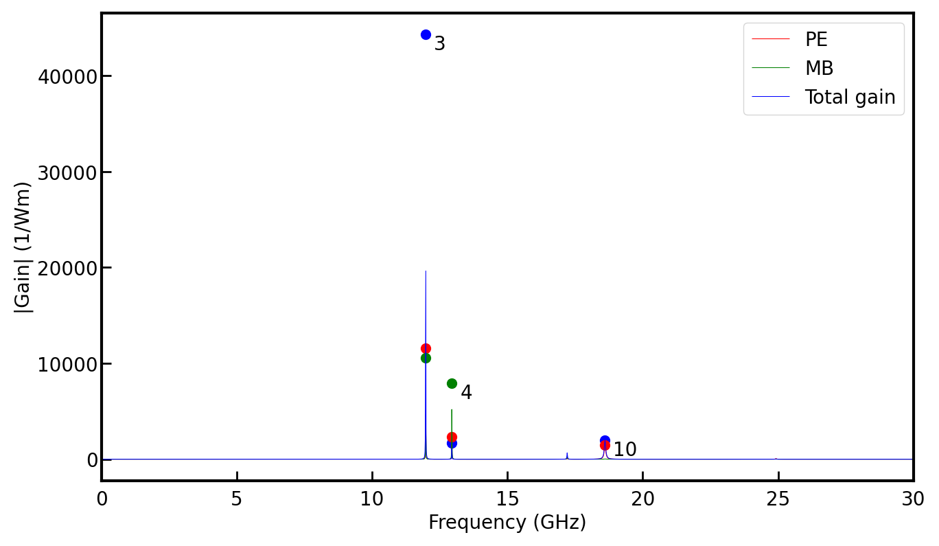
Gain spectrum with anisotropic stiffness model of silicon.

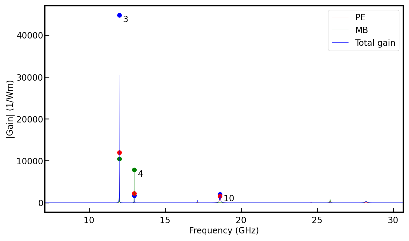
Gain spectrum from Tutorial 2 with isotropic stiffness model of silicon.

5.3.4. Tutorial 11 – Two-layered ‘Onion’

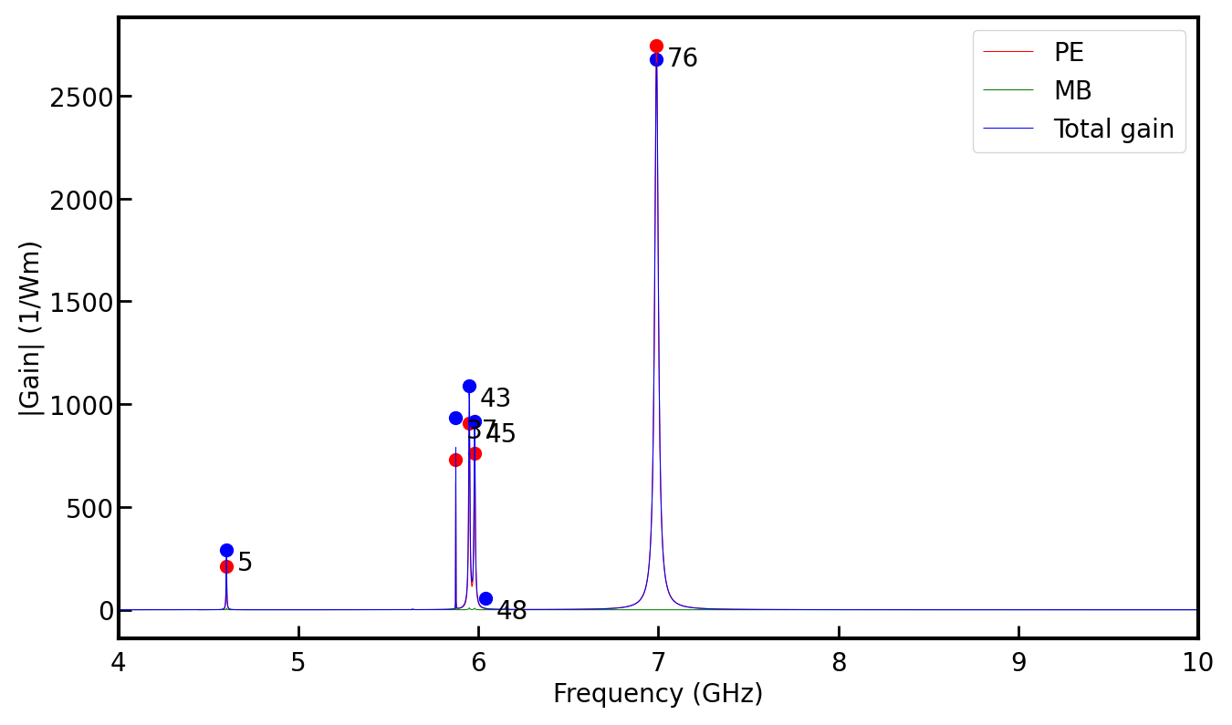
This tutorial, contained in sim-tut_11a-onion2.py demonstrates use of a two-layer onion structure for a backward intra-modal SBS configuration. Note that with the inclusion of the background layer, the two-layer onion effectively creates a three-layer geometry with core, cladding, and background surroundings. This is the ideal structure for investigating the cladding modes of an optical fibre. It can be seen by looking through the optical mode profiles in tut_11a-fields/EM*.png that this particular structure supports five cladding modes in addition to the three guided modes (the \(\mbox{TM}_0\) mode is very close to cutoff).

Next, the gain spectrum and the mode profiles of the main peaks indicate as expected, that the gain is optimal for modes that are predominantly longitudinal in character.

The accompanying tutorial sim-tut_11b-onion3.py introduces one additional layer and would be suitable for studying the influence of the outer polymer coating of an optical fibre or depressed cladding W fibre.

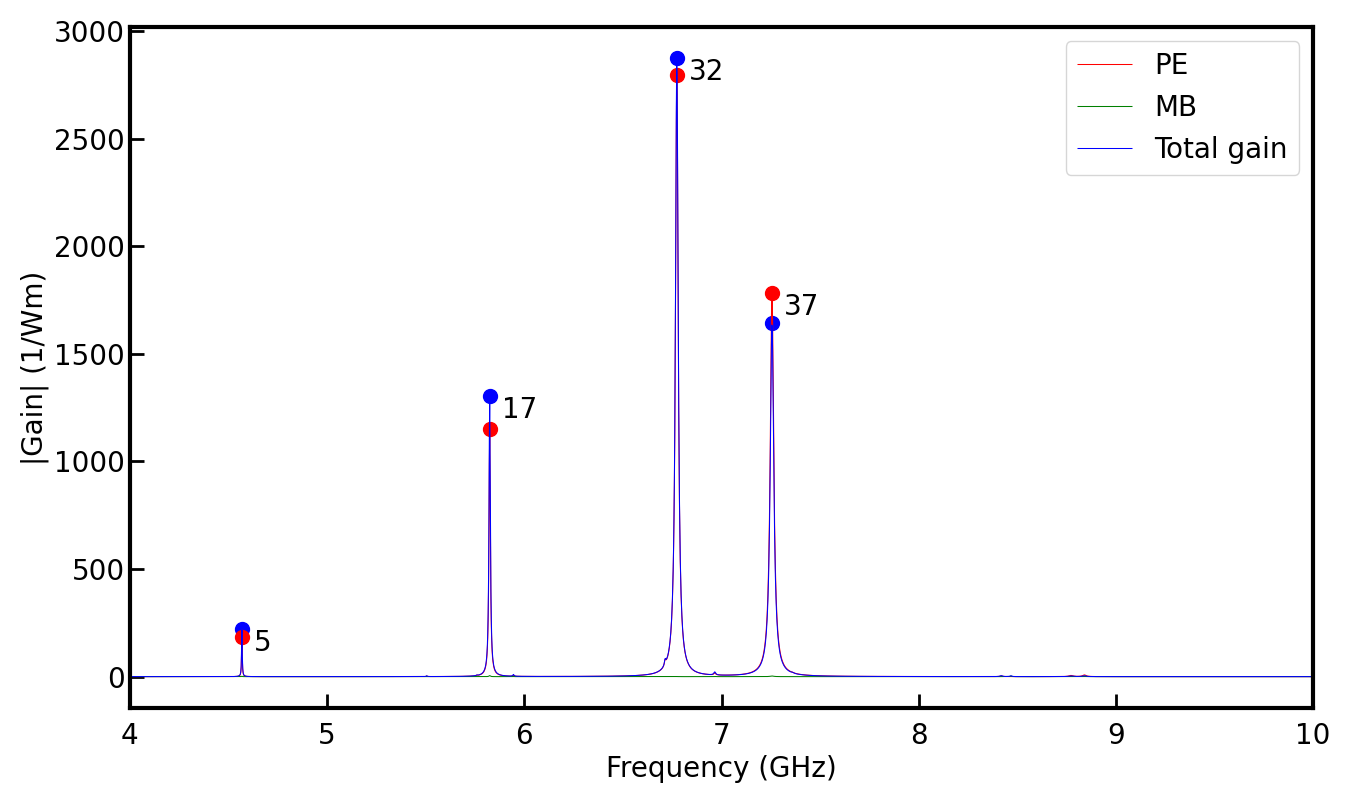
Gain spectrum for the two-layer structure in tut_11a.

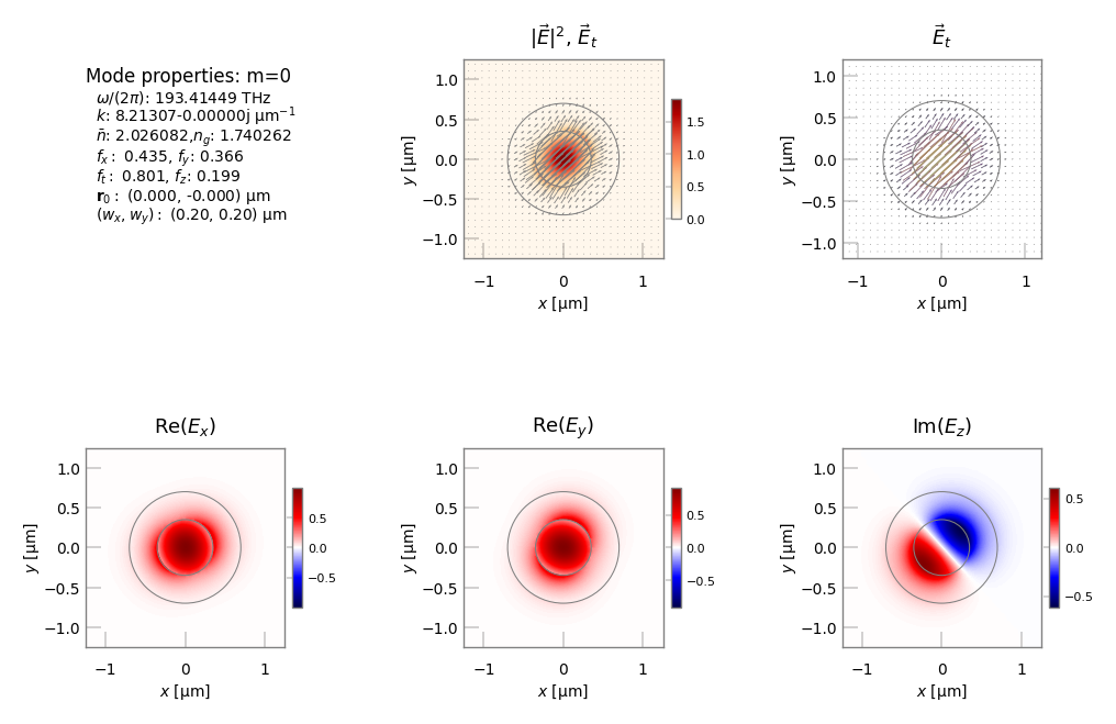
Mode profile for fundamental optical mode.

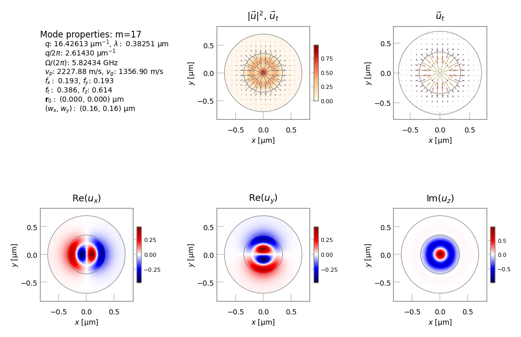
Mode profile for acoustic mode 17.

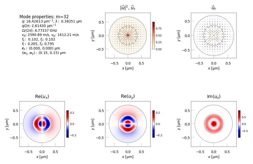
Mode profile for acoustic mode 32.

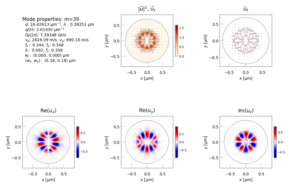
Mode profile for acoustic mode 39.

Gain spectrum for the three-layer structure in tut_11b.

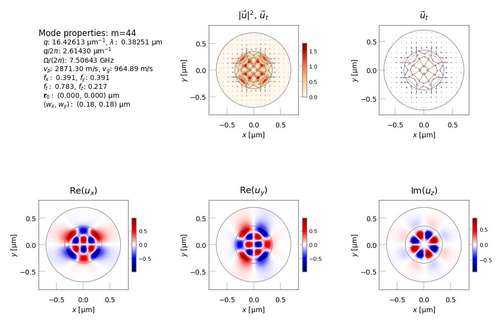
Mode profile for acoustic mode 44.

Mode profile for acoustic mode 66.

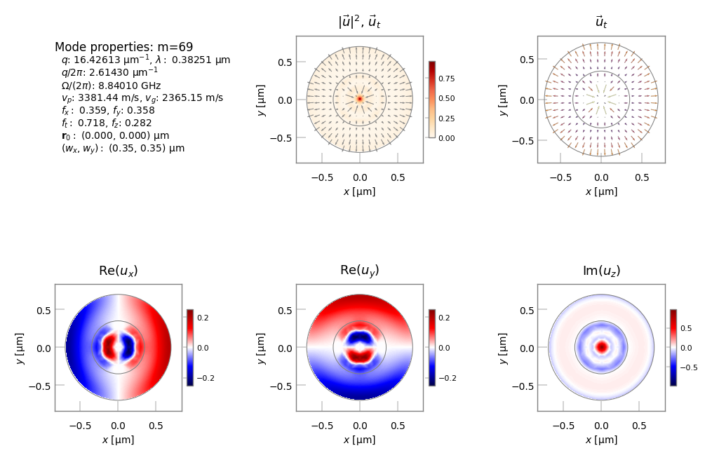
Mode profile for acoustic mode 66.

5.3.5. Tutorial 12 – Validating the calculation of the EM dispersion of a two-layer fibre

How can we be confident that NumBAT’s calculations are actually correct? This tutorial and the next one look at rigorously validating some of the modal calculations produced by NumBAT.

This tutorial, contained in sim-tut_12.py, compares analytic and numerical calculations for the dispersion relation of the electromagnetic modes of a cylindrical waveguide. This can be done in both a low-index contrast (SMF-28 fibre) and high-index contrast (silicon rod in silica) context. We calculate the effective index \(\bar{n}\) and normalised waveguide parameter \(b=(\bar{n}^2-n_\text{cl}^2)/(n_\text{co}^2-n_\text{cl}^2)\) as a function of the normalised freqency \(V=k a \sqrt{n_\text{co}^2-n_\text{cl}^2}\) for radius \(a\) and wavenumber \(k=2\pi/\lambda\). As in several previous examples, this is accomplished by a scan over the wavenumber \(k\).

The numerical results (marked with crosses) are compared to the modes found from the roots of the rigorous analytic dispersion relation (solid lines). We also show the predictions for the group index \(n_g=\bar{n} + V \frac{d\bar{n}}{dV}\). The only noticeable departures are right at the low \(V\)-number regime where the fields become very extended into the cladding and interact significantly with the boundary. The results could be improved in this regime by choosing a larger domain at the expense of a longer calculation.

As this example involves the same calculation at many values of the wavenumber \(k\), we again use parallel processing techniques. However, in this case we demonstrate the use of threads (multiple simultaneous strands of execution within the same process) rather than a pool of separate processes. Threads are light-weight and can be started more efficiently than separate processes. However, as all threads share the same memory space, some care is needed to prevent two threads reading or writing to the same data structure simultaneously. This is dealt with using the helper functions and class in the numbattools.py module.

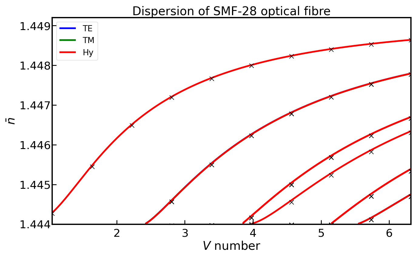
Optical effective index as a function of normalised frequency for SMF-28 fibre.

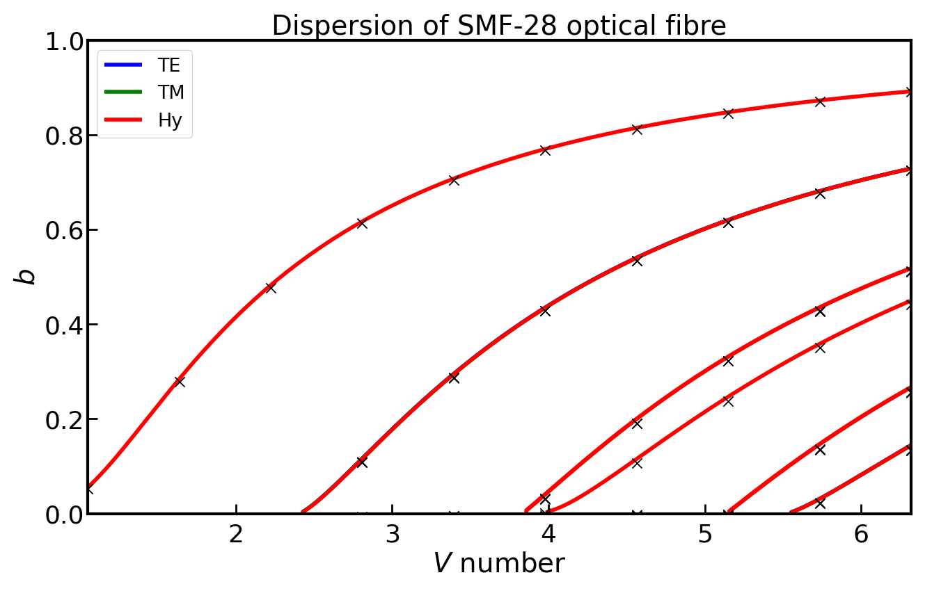
Optical normalised waveguide parameter as a function of normalised frequency for SMF-28 fibre.

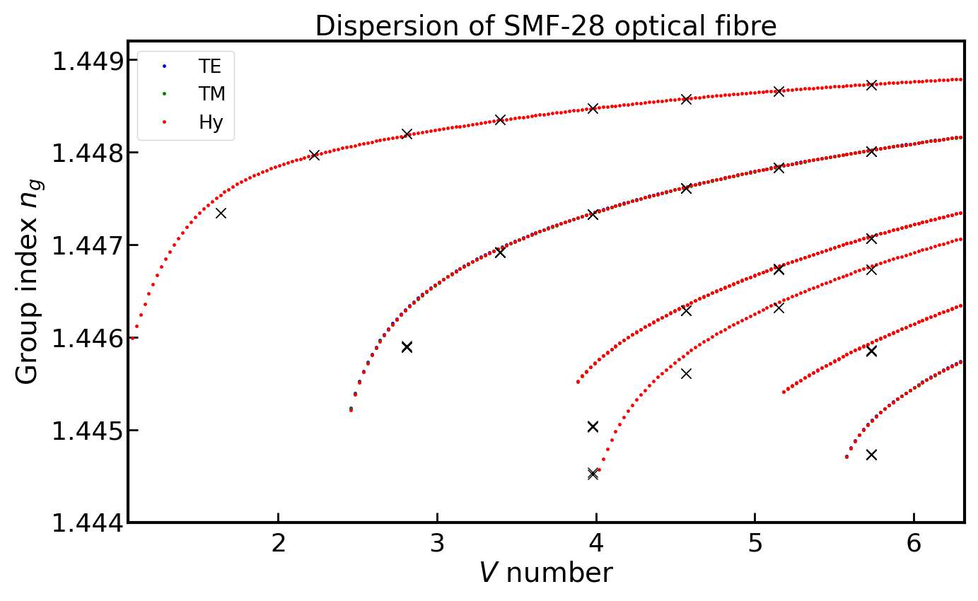
Optical group index \(n_g=\bar{n} + V \frac{d\bar{n}}{dV}\) as a function of normalised frequency for SMF-28 fibre.

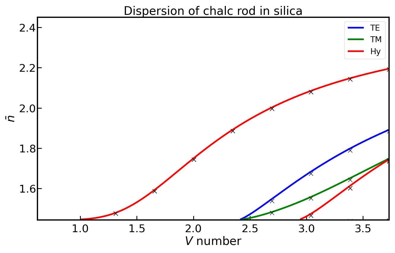
Optical effective index as a function of normalised frequency for silicon rod in silica.

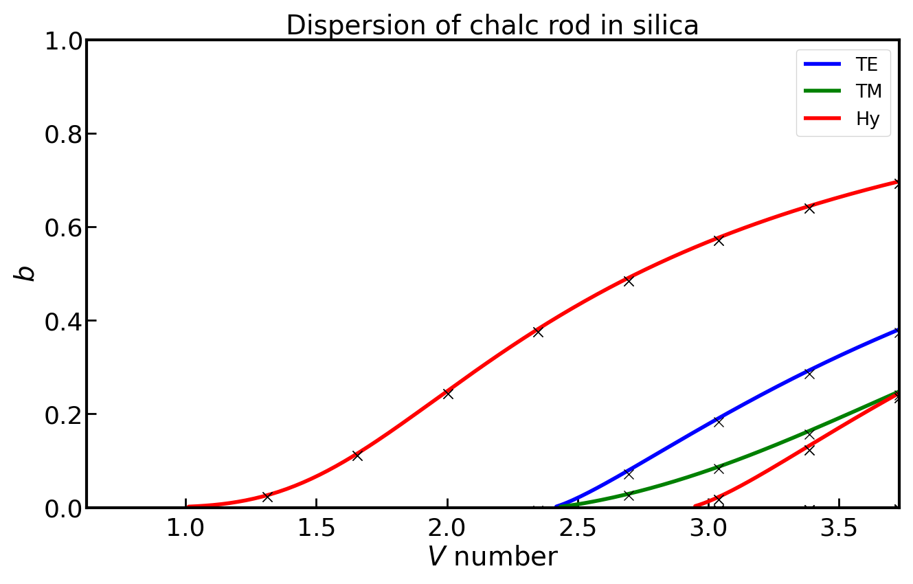
Optical normalised waveguide parameter as a function of normalised frequency for silicon rod in silica.

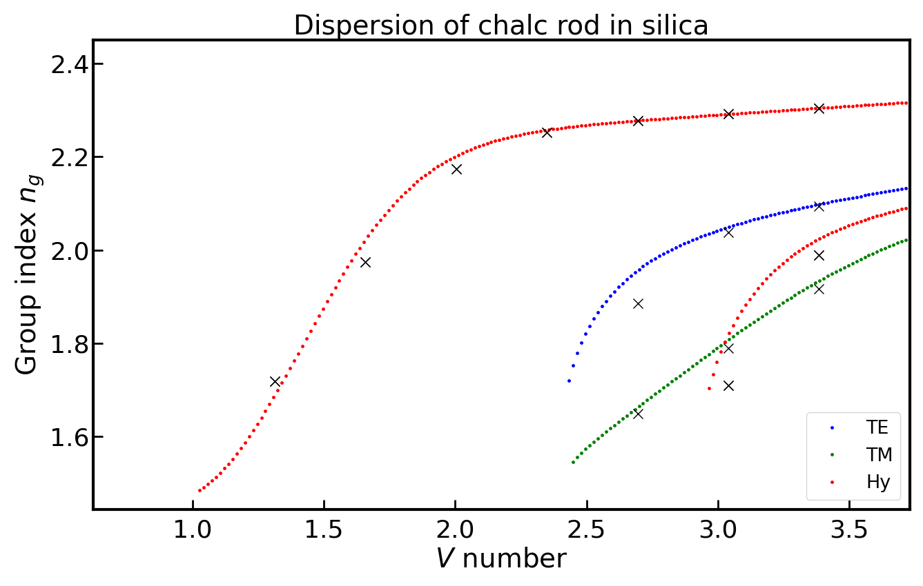
Optical group index \(n_g=\bar{n} + V \frac{d\bar{n}}{dV}\) as a function of normalised frequency for silicon rod in silica.

5.3.6. Tutorial 13 – Validating the calculation of the dispersion of an elastic rod in vacuum

The tutorial sim-tut_13.py performs the same kind of calculation as in the previous tutorial for the acoustic problem. In this case there is no simple analytic solution possible for the two-layer cylinder. Instead we create a structure of a single elastic rod surrounded by vacuum. NumBAT removes the vacuum region and imposes a free boundary condition at the boundary of the rod. The modes found are then compared to the analytic solution of a free homogeneous cylindrical rod in vacuum.

We find excellent agreement between the analytical (coloured lines) and numerical (crosses) results. Observe the existence of two classes of modes with azimuthal index \(p=0\), corresponding to the pure torsional modes, which for the lowest band propagate at the bulk shear velocity, and the so-called Pochammer hybrid modes, which are predominantly longitudinal, but must necessarily involve some shear motion to satisfy mass conservation.

It is instructive to examine the mode profiles in tut_13-fields and track the different field profiles and degeneracies found for each value of \(p\). By basic group theory arguments, we know that every mode with \(p\ne 0\) must come as a degenerate pair and this is satisfied to around 5 significant figures in the calculated results. It is interesting to repeat the calculation with a silicon (cubic symmetry) rod rather than chalcogenide (isotropic). In that case, the lower symmetry of silicon causes splitting of a number of modes, so that a larger number of modes are found to be singly degenerate, though invariably with a partner state at a nearby frequency.

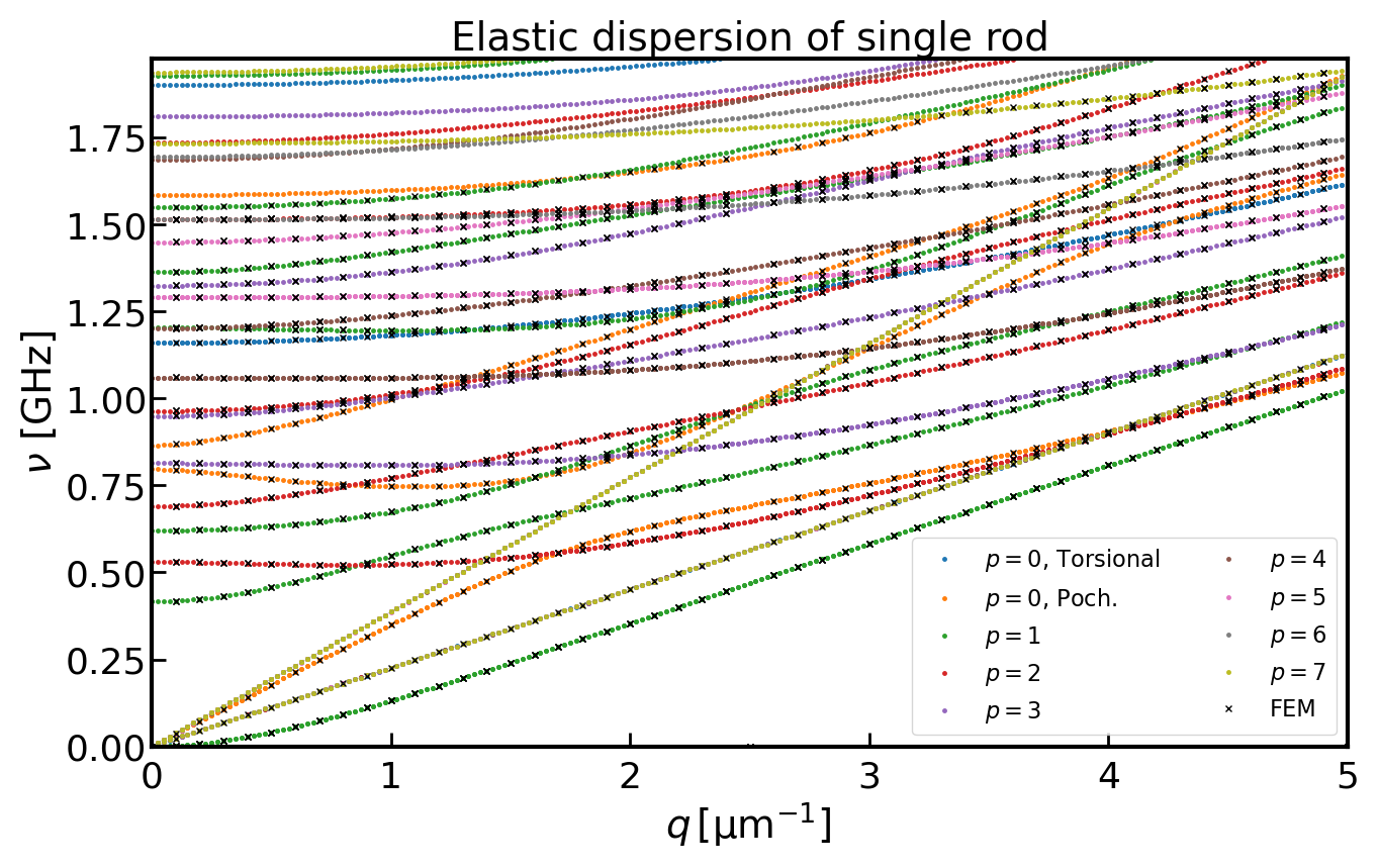
Elastic frequency as a function of normalised wavenumber for a chalcogenide rod in vacuum.

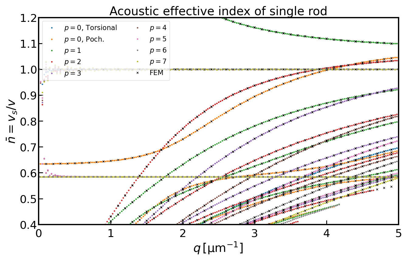
Elastic “effective index” defined as the ratio of the bulk shear velocity to the phase velocity \(n_\text{eff}=V_s/V\), for a chalcogenide rod in vacuum.

5.3.7. Tutorial 14 – Multilayered ‘Onion’

** This tutorial is under development. Expect it to fail.**

This tutorial, contained in sim-tut_14-multilayer-fibre.py shows how one can create a circular waveguide with many concentric layers of different thickness. In this case, the layers are chosen to create a concentric Bragg grating of alternating high and low index layers. As shown in C. M. de Sterke, I. M. Bassett and A. G. Street, “Differential losses in Bragg fibers”, J. Appl. Phys. 76, 680 (1994), the fundamental mode of such a fibre is the fully azimuthally symmetric \(\mathrm{TE}_0\) mode rather than the usual \(\mathrm{HE}_{11}\) quasi-linearly polarised mode that is found in standard two-layer fibres.

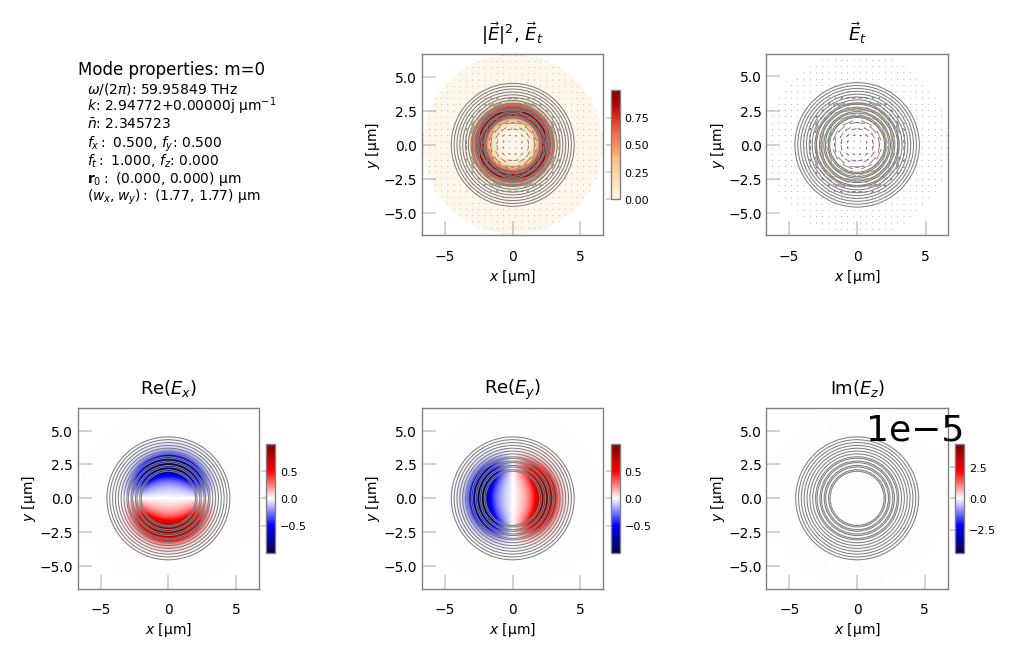
Fundamental electromagnetic mode profile for the concentric Bragg fibre.

5.3.8. Tutorial 15 – Coupled waveguides

This tutorial, contained in tutorials/sim-tut_14-coupled-wg.py demonstrates the supermode behaviour of both electromagnetic and elastic modes in a pair of closely adjacent waveguides.