9. Numerical formulation of the finite element problems

9.1. Introduction

In this chapter we provide some detailed information on how the finite element problems defined in chapter Background theory are expressed as numerical problems that can be solved by standard matrix libraries.

We start with the elastic problem which is somewhat easier to understand since it is formulated with a simpler of elements.

9.2. Elastic modal problem

Recall from Background theory that the elastic wave equation has the form

\[\nabla \cdot \bar{T} + \Omega^2 \rho(x,y) \vec u = 0,\]

where we seek modal eigensolutions \((\vecu_n(\vecrt) e^{i q z}, \Omega_n(q_z))\) for the elastic displacement vector field \(\vecU(\vecr)\):

\[\vec U(\vecr) = b \, \vec u_n(\vecrt) e^{i (qz-\Omega_n(q) t) } + b^* \, \vec u_n^*(\vecrt) e^{-i (qz-\Omega_n(q) t) },\]

where the position vectors are defined \(\vecr \equiv(\vecrt, z)\equiv(x,y,z)\). Refer to chapter Background theory for complete definitions of the density \(\rho(\vecrt)\), the rank-2 stress tensor \(\bar{T}\), and its connection with the stiffness tensor \(\mathbf{c}\) and strain tensor \(\bar{S}\).

In the so-called weak-formulation of this eigenproblem, we seek pairs \((\vecu(\vecrt) e^{i q z}, \Omega(q_z))\) so that for all “test” functions \(\vecv(\vecr)\), the following integral equation holds

\[\int_A \vecv^*(\vecr) \cdot \left( \nabla \cdot \bar{T} + \Omega^2 \rho \vecu(\vecr)\right) \, \dA = 0.\]

9.2.1. Defining the FEM formulation

The weak form equation is a general mathematical statement that softens potential singularities in the original differential equation.

To develop a finite-element numerical algorithm of this statement, the functions \(\vecu(\vecr)\) and \(\vecv(\vecr)\) are expanded in a finite set of \(N\) basis functions \(g_m(\vecrt)\):

\[\begin{split}\vecu(\vecrt) & = \sum_{m=1}^N \begin{bmatrix} u_{m,x} \\ u_{m,y} \\ u_{m,z} \end{bmatrix} g_m(\vecrt) \\ & = \sum_{m=1}^N \sum_{\sigma=x,y,z} u_{m,\sigma} \, g_m(\vecrt) \bfe_{\sigma} \\\end{split}\]

for some set of coefficients \(\vecu_h = (u_{1,x},u_{1,y},u_{1,z},u_{2,x},u_{2,y},u_{2,z},\dots ,u_{N,x},u_{N,y},u_{N,z})\), with separate coefficients for each Cartesian component of the field. Here, \(\bfe_{\sigma}\) stands for the Cartesian unit vectors \(\hat{x}, \hat{y}, \hat{z}\).

Note that the basis functions are scalar and each component of the displacement field is represented by a distinct degree of freedom. (This could be written in a vector notation defining \(\vec g_{m,\sigma}(\vecrt) = g_m(\vecrt) \bfe_\sigma\), but there is no particular advantage in doing so.) Later, we see that this is handled differently in the electromagnetic problem where the basis functions are chosen to have a non-trivial vector character.

9.2.1.1. FEM basis functions

In NumBAT, the \(g_m(\vecrt)\) are chosen as piecewise quadratic polynomials defined on each domain of an irregularly shaped triangular grid. These basis functions or elements are known as Lagrange P2 polynomials illustrated in the figure below.

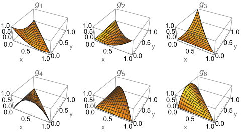
Lagrange P2 polynomial scalar basis functions.

The standard polynomials are defined on the “unit” triangle with vertices or nodes at \(\vecr_1=(0,0)\), \(\vecr_2=(1,0)\), and \(\vecr_3=(0,1)\). Three additional nodes 4,5,6 label the mid-points at \(\vecr_4= (\frac{1}{2},0)\), \(\vecr_5= (0,\frac{1}{2})\), and \(\vecr_6=(\frac{1}{2},\frac{1}{2})\).

Observe that each polynomial takes the value zero at all nodes except the one corresponding to its label:

\[g_i(\vecr_j) = \delta_{ij},\]

and so frequently we can identify the nodes and basis functions of the same index.

The triangles in the FEM grid have arbitrary shapes and node locations, so that the values and overlap integrals of the functions are calculated for each triangle using an affine transformation.

9.2.1.2. Determining the FEM matrices

The numerical task is to find eigenvector solutions for the vector of coefficients or degrees of freedom \(\vecu_h\).

How many degrees of freedom are there? There are six P2 polynomials for each triangle in the grid. Since most nodes belong to more than one triangle and also due to the application of boundary conditions at the edge of the domain, the precise number of degrees of freedom depends on the exact arrangement of triangles in the FEM grid, but will be of order \(n_\text{dof}=10 n_t\) where \(n_t\) is the number of triangles.

On inserting the field expansion into the weak form integral equation, the eigenproblem ultimately leads to the generalised linear eigenvalue equation (see [1]),

\[\rmK \vecu_h = \Omega^2 \rmM \vecu_h ,\]

where the stiffness \(\rmK\) and mass \(\rmM\) operators capture the details of the waveguide structure. Note that the labels “stiffness” and “mass” are generic FEM terms, and are unrelated to the physical concepts of stiffness tensor and density in our specific elastic problem.

The values in the \(\rmK\) and \(\rmM\) operators are evaluated triangle by triangle. On each triangle, these operators are \(18 \times 18\) matrices (6 nodes with 3 components). Labelling the elements by number \(i=1..6\) and component \(\sigma=x,y,z\), we can write explicit formulae for each matrix element, with the rows associated with the test function \(v\) and the columns with the coefficients of the eigenfunction \(u_n\).

The mass operator comes from the second term in the weak-form wave equation:

\[ \begin{align}\begin{aligned}M_{i,\sigma; j, \tau} &= \int_A \rho(\vecrt) g_i(\vecrt) \vece_\sigma \cdot g_j(\vecrt) \vece_\tau \, \dx\dy\\ &= \delta_{\sigma,\tau} \int_A \rho(\vecrt) g_i(\vecrt) g_j(\vecrt) \, \dx\dy\end{aligned}\end{align} \]

The stiffness operator implements the negative of the first term in the weak-form wave equation (negative since it has been moved to the other side of the equation). It requires a bit more work to evaluate:

\[\begin{split}K[\vecv, \vecu] & = - \int_A \vecv^*(\vecrt) \cdot (\nabla \cdot \bar{T}[\vecu]) \, \dA \\ & = - \int_A v^*_a (\nabla \cdot \bar{T}[\vecu])_a \, \dA \\ & = - \int_A v^*_a (\partial_b T_{ab}) \, \dA \\ & = \int_A (\partial_b v^*_a) T_{ab} \, \dA \\ & = \int_A (\partial_b v^*_a) c_{abcd} S_{cd} \, \dA \\ & = \int_A (\partial_b v^*_a) c_{abcd} \tfrac{1}{2} (\partial_c u_d + \partial_d u_c) \, \dA \\ & = \frac{c_{abcd}}{2}\int_A (\partial_b v^*_a) (\partial_c u_d + \partial_d u_c) \, \dA \\\end{split}\]

Now to find \(K_{i,\sigma;j,\tau}\) we can set \(v_a \to g_i \delta_{a,\sigma} e^{iqz}\), \(u_c \to g_j \delta_{c,\tau} e^{iqz}\) and \(u_d \to g_j \delta_{d,\tau} e^{iqz}\), to obtain

\[\begin{split}K_{i,\sigma;j,\tau} & = \frac{c_{abcd}}{2} \int_A (\partial_b g_i \delta_{a,\sigma} e^{-iqz}) (\partial_c g_j \delta_{d,\tau} e^{iqz} + \partial_d g_j \delta_{c,\tau} e^{iqz}) \, \dA \\ & = \frac{c_{\sigma bcd}}{2} \int_A (\partial_b g_i e^{-iqz}) (\partial_c g_j \delta_{d,\tau} e^{iqz} + \partial_d g_j \delta_{c,\tau} e^{iqz}) \, \dA \\ & = \frac{c_{\sigma bc\tau}}{2} \int_A (\partial_b g_i e^{-iqz}) (\partial_c g_j e^{iqz})\, \dx\dy +\frac{c_{\sigma b\tau d}}{2} \int_A (\partial_b g_i e^{-iqz}) (\partial_d g_j e^{iqz})\, \dx\dy\end{split}\]

Writing the integral \(\int_A f \dA = \langle f \rangle\) these terms can be evaluated as

\[\begin{split}G^{ij}_{b c} & = \langle (\partial_b g_i e^{-iqz}) (\partial_c g_j e^{iqz}) \rangle \\ & = \langle (-iq g_i \delta_{bz} + (\partial_b g_i) (1-\delta_{bz})) (iq g_j \delta_{cz} + (\partial_c g_j) (1-\delta_{cz})) \rangle \\ &= \langle q^2 g_i g_j \delta_{bz} \delta_{cz} -iq g_i (\partial_c g_j) \delta_{bz} (1-\delta_{cz}) \\ & ~~~~ + iq (\partial_b g_i) g_j (1-\delta_{bz}) \delta_{cz} + (\partial_b g_i)(\partial_c g_j) (1-\delta_{bz}) (1-\delta_{cz}) \rangle \\ &= \begin{bmatrix} \langle (\partial_x g_i) (\partial_x g_j) \rangle & \langle (\partial_x g_i) (\partial_y g_j) \rangle & \langle (\partial_x g_i) (i q g_j) \rangle\\ \langle (\partial_y g_i) (\partial_x g_j) \rangle & \langle (\partial_y g_i) (\partial_y g_j) \rangle & \langle (\partial_y g_i) (i q g_j) \rangle\\ \langle (-iq g_i) (\partial_x g_j) \rangle & \langle (-iq g_i) (\partial_y g_j) \rangle& q^2 \langle g_i g_j \rangle \end{bmatrix}_{bc} \\ &= \begin{bmatrix} \langle g_{i;x} g_{j;x} \rangle & \langle g_{i;x} g_{j;y} \rangle & i q \langle g_{i;x} g_j \rangle \\ \langle g_{i;y} g_{j;x}\rangle & \langle g_{i;y} g_{j;y} \rangle & i q \langle g_{i;y} g_j \rangle \\ -iq \langle g_i g_{j;x}\rangle & -iq \langle g_i g_{j;y} \rangle & q^2 \langle g_i g_j \rangle \end{bmatrix}_{bc}\end{split}\]

which at last gives

\[\begin{split}K_{i,\sigma;j,\tau} & = \frac{c_{\sigma bc \tau}}{2} G^{ij}_{bc} + \frac{c_{\sigma b \tau d}}{2} G^{ij}_{bd} \\ & = \frac{1}{2} \left( c_{\sigma bc \tau} G^{ij}_{bc} + c_{\sigma b \tau c} G^{ij}_{bc} \right)\\ & = \frac{1}{2} \left( c_{\sigma bc \tau} G^{ij}_{bc} + c_{\sigma b c\tau } G^{ij}_{bc} \right)\\ & = c_{\sigma bc \tau} G^{ij}_{bc}\end{split}\]

using the symmetries \(c_{ijkl}=c_{jikl}=c_{ijlk}\).

Evaluating a couple of these elements using the Voigt notation for the stiffness tensor gives

\[ \begin{align}\begin{aligned}\begin{split}K_{x,i;x,j} & = c_{x bc x} G^{ij}_{bc} \\ & = \left [ c_{x xx x} G^{ij}_{xx} + c_{x xy x} G^{ij}_{xy} + c_{x xz x} G^{ij}_{xz} + c_{x yx x} G^{ij}_{yx} + c_{x yy x} G^{ij}_{yy} \right . \\ & ~~~~~~~~ + \left . c_{x yz x} G^{ij}_{yz} + c_{x zx x} G^{ij}_{zx} + c_{x zy x} G^{ij}_{zy} + c_{x zz x} G^{ij}_{zz} \right] \\ & =\left [ C_{11} G^{ij}_{xx} + C_{16} G^{ij}_{xy} + c_{15} G^{ij}_{xz} + c_{66} G^{ij}_{yx} + c_{66} G^{ij}_{yy} \right . \\ & ~~~~~~~~ + \left . c_{65} G^{ij}_{yz} + c_{51} G^{ij}_{zx} + c_{56} G^{ij}_{zy} + c_{55} G^{ij}_{zz} \right ]\end{split}\\\begin{split}K_{x,i;y,j} & = c_{x bc y} G^{ij}_{bc} \\ & = \left [ c_{x xx y} G^{ij}_{xx} + c_{x xy y} G^{ij}_{xy} + c_{x xz y} G^{ij}_{xz} + c_{x yx y} G^{ij}_{yx} + c_{x yy y} G^{ij}_{yy} \right . \\ & ~~~~~~~~ + \left . c_{x yz y} G^{ij}_{yz} + c_{x zx y} G^{ij}_{zx} + c_{x zy y} G^{ij}_{zy} + c_{x zz y} G^{ij}_{zz} \right] \\ &=\left [ C_{16} G^{ij}_{xx} + C_{12} G^{ij}_{xy} + c_{14} G^{ij}_{xz} + c_{66} G^{ij}_{yx} + c_{62} G^{ij}_{yy} \right . \\ & ~~~~~~~~ + \left . c_{64} G^{ij}_{yz} + c_{56} G^{ij}_{zx} + c_{52} G^{ij}_{zy} + c_{55} G^{ij}_{zz} \right ]\end{split}\end{aligned}\end{align} \]

9.2.2. Solving the numerical problem

The entire \(\rmK\) and \(\rmM\) matrices have dimension \(n_\text{dof} \times n_\text{dof}\) and are filled output by performing the above operation for each triangle in turn. But since only degrees of freedom that share a triangle can give nonzero terms, they are overwhelmingly sparse matrices. In NumBAT they are represented using the Compressed Sparse Column (CSC) format. Additional book-keeping is required in that most degrees of freedom are involved in multiple triangles but in each case must be mapped back to their unique row and column.

These matrices are constructed in the source files build_fem_ops_ac.f90 which loops over all triangles and make_elt_femops_ac.f90 which evaluates the operators for one triangle.

This matrix eigenproblem is then solved using standard linear algebra numerical libraries including ARPACK-NG, UMFPACK on top of the LAPACK and BLAS libraries. These libraries are installed separately by the user allowing selection of implementations that are optimal for the local operating system and hardware.

Once the coefficients \(\vecu_h\) are known for a particular mode, they can be interpolated onto a rectangular grid for plotting. Note that evaluation of the key SBS coupling integrals is performed on the original FEM grid for accuracy.

9.3. Electromagnetic problem

We closely follow the exposition in [4].

Expressed in the modal form \(\vecE(\vecr)= [\vecE_t, E_z]e^{i \beta z}\), the wave equation becomes the pair of equations:

\[ \begin{align}\begin{aligned}\nabla_t \times \left(\frac{1}{\mu}(\nabla_t \times \vecE_t) \right) - \omega^2 \epsilon \vecE_t = & \, \beta^2 \frac{1}{\mu} ( \nabla \hE_z- \vecE_t)\\- \nabla_t \cdot (\frac{1}{\mu} \vecE_t) + \nabla_t \cdot(\frac{1}{\mu} \nabla_t \hE_z) + \omega^2 \epsilon \hE_z =& \, 0 ,\end{aligned}\end{align} \]

where for convenience we have introduced \(\hE_z E_z = -E_z/\beta\), and in practice the permeability is always $mu=mu_0$.

In the weak-form formulation, we seek pairs \((\vecE, \beta)\) so that for all test functions \(\vecF(\vecr)\), the following equations hold

\[ \begin{align}\begin{aligned}\left(\frac{1}{\mu} (\nabla_t \times \vecE_t), \nabla_t \times \vecF_t\right) - \omega^2 \left(\epsilon \vecE_t, \vecF_t\right) = \, \beta^2 \left(\frac{1}{\mu} ( \nabla \hE_z- \vecE_t), \vecF_t \right)\\\left(\frac{1}{\mu} \vecE_t,\nabla_t F_z \right) - \left(\frac{1}{\mu} \nabla_t \hE_z, \nabla_t F_z \right) + \omega^2 \left (\epsilon \hE_z, F_z \right ) = \, 0 ,\end{aligned}\end{align} \]

where for arbitrary terms \(\vec A, \vec B\) the inner product is defined

\[(\vec A, \vec B) = \int (\vec B)^* \cdot (\vec A) \, \dA.\]

9.3.1. Defining the FEM formulation

The basis sets used to construct the FEM formulation are more involved than for the elastic problem, with the transverse and longitudinal components represented differently. We introduce transverse vector basis functions \(\vphi_i(x,y)\) and scalar longitudinal functions \(\psi_i(x,y)\) so that a general field has the form

\[\begin{split}\vecE = & \vecE_t + \unitz E_z \\ = & \sum_{i=1}^{M} e_{t,i} \, \vphi_i(\vecr) + \unitz \sum_{i=1}^{N} \he_{z,i} \, \psi_i(\vecr) \\ = & [\vphi_1, \vphi_2, \ldots, \vphi_M,\psi_1, \psi_2, \ldots, \psi_N, ] \begin{bmatrix} e_{t,1} \\ e_{t,2} \\ \ldots \\ e_{t,M} \\ \he_{z,1} \\ \he_{z,2} \\ \ldots \\ \he_{z,N} \end{bmatrix} \\ = & [\bvphi ; \unitz \bpsi] \begin{bmatrix} \bfe_t \\ \bfhez \end{bmatrix}\end{split}\]

9.3.1.1. The basis functions

The longitudinal component of the field is represented by 10 P3 Lagrange polynomials. These have nodes at the three vertices, six one-third points along each edge, and the barycentre of the triangle at \(\vecr_{10}=(\frac{1}{3},\frac{1}{3})\):

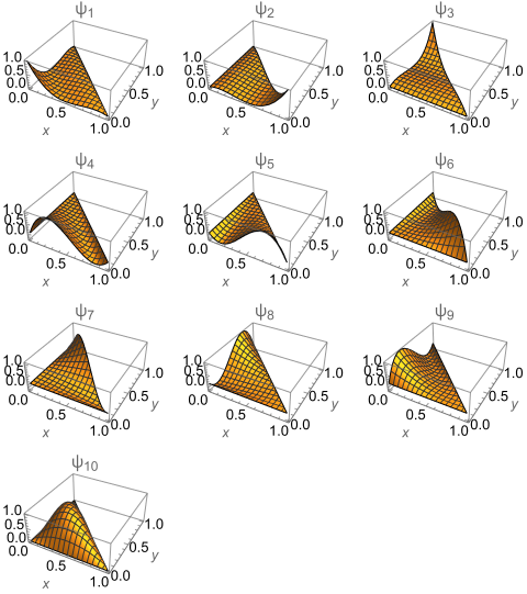
Lagrange P3 polynomial scalar basis functions.

The transverse part of the field is represented by 12 basis functions composed from products of P2 polynomials and gradients of P1 polynomials. Three functions (shown in each row in the figure below) are associated with each of the barycentre and the three edge mid-points.

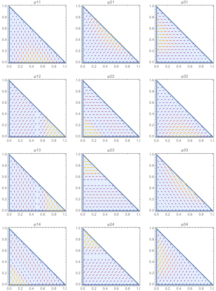
Lagrange P3 polynomial scalar basis functions.

Hence in the basis function expansion above, we have \(M=12\) and \(N=10\).

9.3.1.2. Determining the FEM matrices

An arbitrary inner product \((\calL_1 E, \calL_2 F)\) with \(\calF = a \vphi_m+ b\psi_m \unitz\) where \(a\) and \(b\) are zero or one, expands to

\[\begin{split}(\calL_1 \vecE, \calL_2 \vecF) = & \int (\calL_2 \vecF)^* \cdot (\calL_1 \vecE) \, \dA \\ = & \int (\calL_2 a \vphi_m + b \psi_m \unitz)^* \cdot ( \calL_1 [\bvphi ; \unitz \bpsi] \begin{bmatrix} \bfe_t \\ \mathbf{\hat{e}}_z \end{bmatrix} ) \\ = & a \int (\calL_2 \vphi_m )^* \cdot ( \calL_1 \vphi_n ) \, \dA \, e_{t,n} + b \int (\calL_2 \psi_m \unitz )^* \cdot ( \calL_1 \vphi_n ) \, \dA\, e_{t,n} \\ ~ & + a\int (\calL_2 \vphi_m )^* \cdot ( \calL_1 \psi_n \unitz ) \, \dA\,\he_{z,n} + b \int (\calL_2 \psi_m \unitz )^* \cdot ( \calL_1 \psi_n \unitz ) \, \dA\, \he_{z,n} \\ = & \calL_{tt} \bfe_{t} + \calL_{zt} \bfe_{z} + \calL_{tz}\bfhez + \calL_{zz} \bfhez.\end{split}\]

With these definitions we can identify the matrices

\[\begin{split}K_{mn} = & \int \left [ (\nabla_t \times \vphi_m )^* \cdot \frac{1}{\mu} (\nabla_t \times \vphi_n) - \omega^2 \vphi_m ^* \cdot ( \epsilon \vphi_n) \right ] \, \dA \\ K_{zt} = & \int (\nabla_t \psi_m )^* \cdot \frac{1}{\mu} \vphi_n \, \dA \\ K_{zz} = & \omega^2 \int \psi_m ^* \cdot \epsilon \psi_n \, \dA \\ M_{tt} = & - \int \vphi_m ^* \cdot \vphi_n \, \dA \\\end{split}\]

Then the eigenproblem to be solved is the generalised linear problem

\[\begin{split}\begin{bmatrix} [K_{tt}] &[ 0] \\ [K_{zt}] & [K_{zz}] \end{bmatrix} \begin{bmatrix} e_{t,h} \\ e_{z,h} \end{bmatrix} = \beta^2 \begin{bmatrix} [M_{tt}] &[K_{zt}]^T \\ [0] & [0] \end{bmatrix} \begin{bmatrix} e_{t,h} \\ e_{z,h} \end{bmatrix} .\end{split}\]

By swapping the sides of the second row, the two matrices involved become symmetric:

\[\begin{split}\begin{bmatrix} [K_{tt}] &[ 0] \\ [0] & [0] \end{bmatrix} \begin{bmatrix} e_{t,h} \\ e_{z,h} \end{bmatrix} = \beta^2 \begin{bmatrix} [M_{tt}] &[K_{zt}]^T \\ [K_{zt}] & [K_{zz}] \end{bmatrix} \begin{bmatrix} e_{t,h} \\ e_{z,h} \end{bmatrix},\end{split}\]

which is ideally posed to solve using standard numerical libraries.