5.2.1. Tutorial 2 – SBS Gain Spectra

The first example we met in the previous chapter only printed numerical data to the screen with no graphical output. This example, contained in <NUMBAT>/examples/tutorials/sim-tut_02-gain_spectra-npsave.py considers the same silicon-in-air structure but adds plotting of fields, gain spectra and techniques for saving and reusing data from earlier calculations.

As before, move to the <NUMBAT>/examples/tutorials directory, and then run the calculation by entering:

$ python3 sim-tut_02-gain_spectra-npsave.py

Or you can take advantage of the Makefile provided in the directory and just type:

$ make tut02

Some of the tutorial problems can take a little while to run, especially if your computer is not especially fast. To save time, you can run most problems with a coarser mesh at the cost of somewhat reduced accuracy, by adding the flag fast=1 to the command line:

$ python3 sim-tut_02-gain_spectra-npsave.py fast=1

Or using the makefile technique, simply

$ make ftut02

The calculation should complete in a minute or so. You will find a number of new files in the current directory beginning with the prefix tut_02 (or ftut_02 if you ran in fast mode).

5.2.1.1. Gain Spectra

The Brillouin gain spectra and plotted using the functions integration.get_gains_and_qs() and GainProps.plot_spectra(). The results are contained in the file tut_02-gain_spectra.png which can be viewed in any image viewer. On Linux, for instance you can use

$ eog tut_02_gain_spectra.png

to see this image:

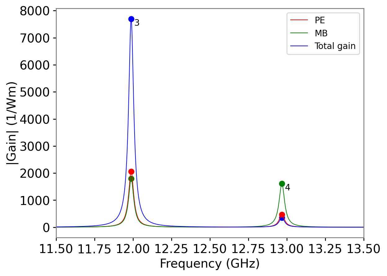
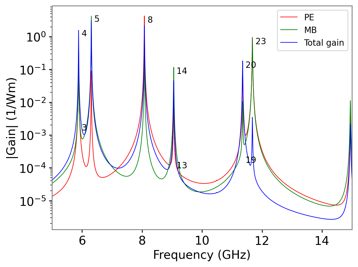
Gain spectrum in tut_02-gain_spectra.png showing gain due to the photoelastic effect, gain due to moving boundary effect, and the total gain. The numbers near the main peaks identify the acoustic mode associated with the resonance.

Note how the different contributions from the photoelastic and moving-boundary effects are visible. In some cases, the total gain (blue) may be less than one or both of the separate effects if the two components act with opposite sign. (This is because the different contributions to the gain add as complex amplitudes). JOSA-B Tutorial Paper and Additional Literature Examples. (See Literature example 1 in the chapter Additional Literature Examples for an interesting cexample of this phenomenon.)

Note also that prominent resonance peaks in the gain spectrum are labelled with the mode number \(m\) of the associated acoustic mode. This makes it easy to find the spatial profile of the most relevant modes (see below).

5.2.1.2. Mode Profiles

The choice of parameters for plot_gain_spectra() has caused several other files to be generated showing a zoomed-in version near the main peak, and the whole spectrum on \(\log\) and dB scales:

Zoom-in of the gain spectrum in the previous figure in the file tut_02-gain_spectra_zoom.png .

Gain spectrum viewed on a log scale in the field tut_02-gain_spectra-logy.png .

This example has also generated plots of some of the electromagnetic and acoustic modes that were found in solving the eigenproblems. These are created using the calls to plot_modes() and stored in the sub-directory tut_02-fields.

Note that a number of useful parameters are also displayed at the top-left of each mode profile. These parameters can also be extracted using a range of function calls on a Mode object (see the API docs). Observe that NumBAT chooses the phase of the mode profile such that the transverse components are real. Note that the \(E_z\) component is \(\pi/2\) out of phase with the transverse components. (Since the structure is lossless, the imaginary parts of the transverse field, and the real part of \(E_z\) are zero). The same is true for the magnetic field components and the elastic displacement fields.

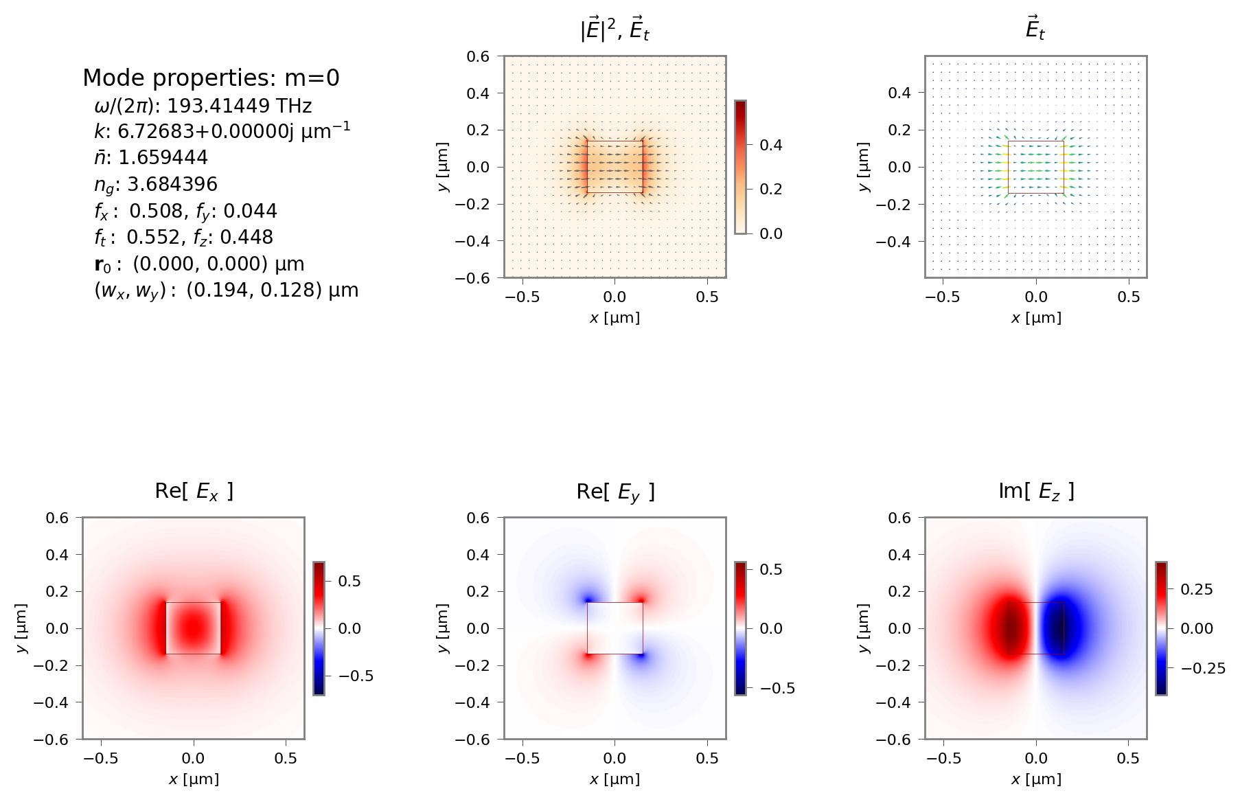
Electric field profile of the fundamental (\(m=0\)) optical mode profile stored in tut_02-fields/EM_E_mode_00.png. The plots show the modulus of the whole electric field \(|{\vec E}|^2\), a vector plot of the transverse field \({\vec E}_t=(E_x,E_y)\), and the three components of the electric field.

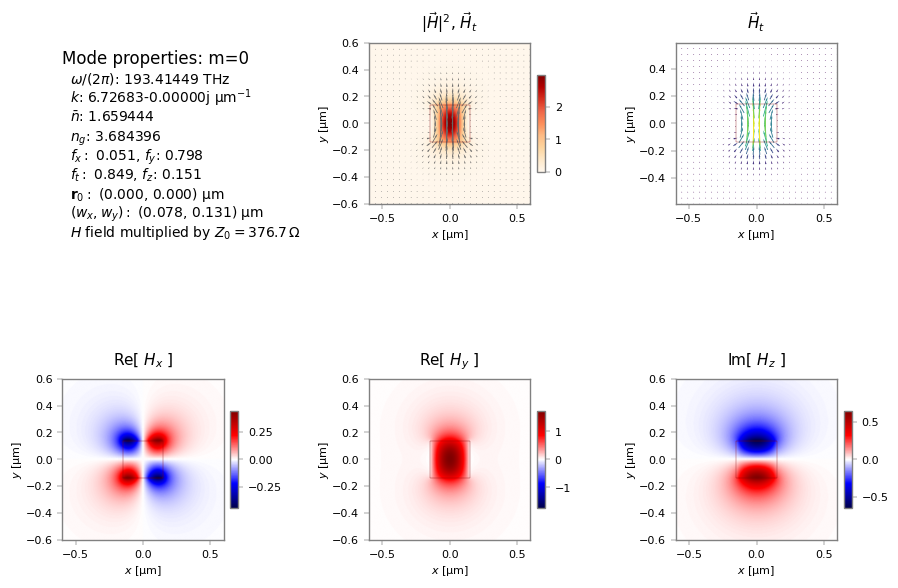
Magnetic field profile of the fundamental (\(m=0\)) optical mode profile showing modulus of the whole magnetic field \(|{\vec H}|^2\), vector plot of the transverse field \({\vec H}_t=(H_x,H_y)\), and the three components of the magnetic field.

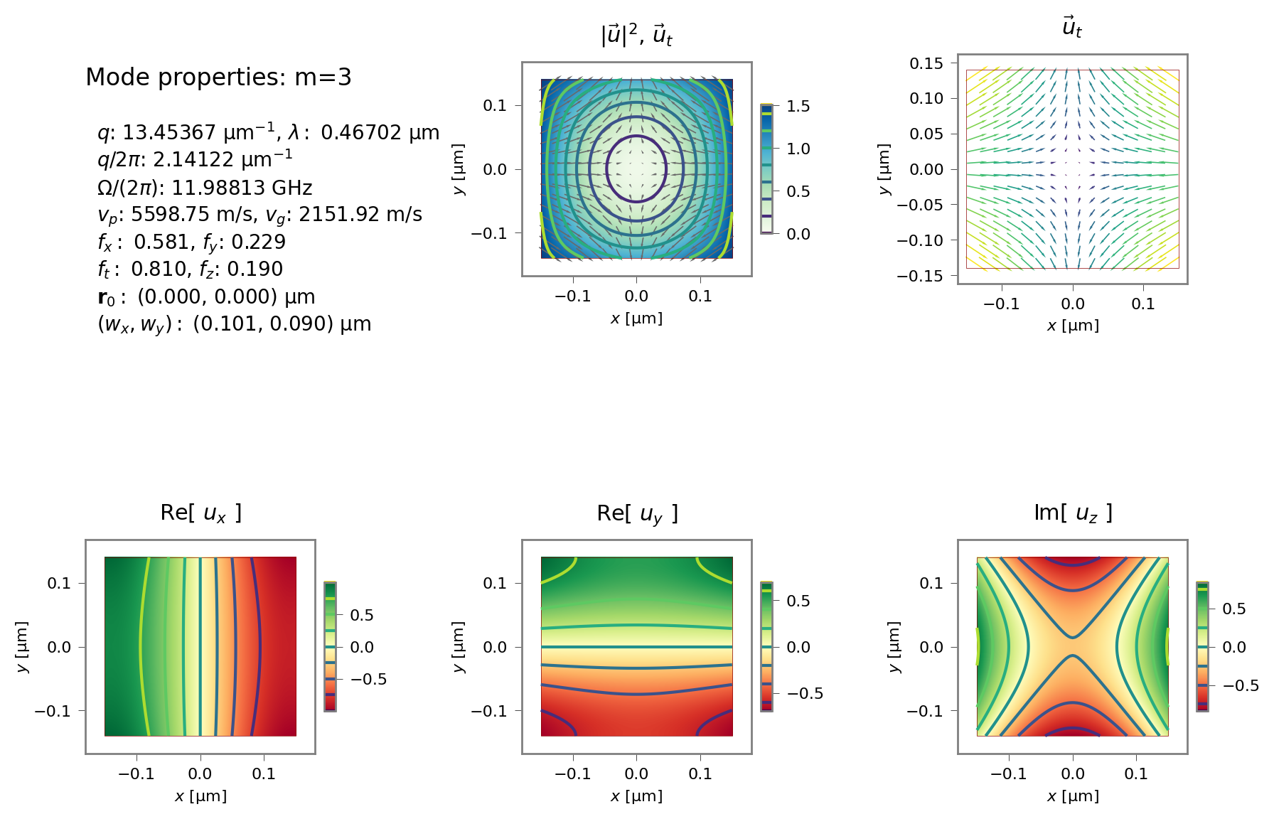
Displacement field \(\vec u(\vec r)\) of the \(m=3\) acoustic mode with gain dominated by the moving boundary effect (green curve in gain spectra). As with the optical fields, the \(u_z\) component is \(\pi/2\) out of phase with the transverse components. Note that the frequency of \(\Omega/(2\pi)=11.99\) GHz (listed in the upper-left corner) corresponds to the first peak in the gain spectrum.

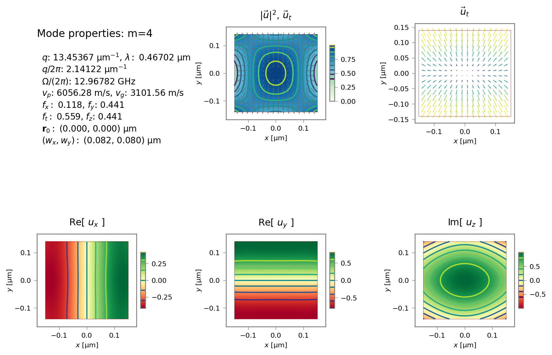
Displacement field \(\vec u(\vec r)\) of the \(m=4\) acoustic mode with gain dominated by the photo-elastic effect (red curve in gain spectra). Note that the frequency of \(\Omega/(2\pi)=13.45\) GHz corresponds to the second peak in the gain spectrum.

A number of plot settings including colormaps and font sizes can be controlled using the numbat.toml file. This is discussed in Additional details.

5.2.1.3. Miscellaneous comments

Here are some further elements to note about this example:

1. When using the fast= mode, the output data and fields directory begin with ftut_02 rather than tut_02.

2. It is frequently useful to be able to save and load the results of simulations to adjust plots without having to repeat the entire calculation. Here the flag reuse_old_fields determines whether the calculation should be done afresh and use previously saved data. This is performed using the save_simulation() and load_simulation() calls.

3. Plots of the modal field profiles are obtained using the plot_modes methods of the EM and elastic sim result structure. Both electric and magnetic fields can be selected using EM_E or EM_H as the value of the field_type argument. The selection of mode numbers to be plotted is specified by ivals. These fields are stored in a folder tut_02-fields/ within the tutorial folder. Later we will see how an alternative approach in which we extract a Mode object from a Simulation which represents a single mode that is able to plot itself. This can be more convenient.

4. The overall amplitude of the modal fields is arbitrary. In NumBAT, the maximum value of the electric field is normalised to be 1.0, and this may be interpreted as a quantity in units of V/m, \(\sqrt{\mathrm{W}}\) or other units as desired. Importantly, when plotted, the magnetic field \(\vec H(\vec r)\) is multiplied by the impedance of free space \(Z_0=\sqrt{\mu_0/\epsilon_0}\) so that the plotted quantities \(Z_0 \vec H(\vec r)\) and \(\vec E(\vec r)\) have the same units, and the relative amplitudes of the electric and magnetic field plots can be compared meaningfully.

5. The suppress_imimre option suppresses plotting of the \(\text{Im}[F_x]\), \(\text{Im}[F_y]\) and \(\text{Re}[F_z]\) components of the fields \(\vec F \in [\vec E, \vec H, \vec u]\). In a lossless non-leaky problem, these fields should normally be zero at all points and therefore not useful to plot.

6. By default, plots are exported as png format. This can be adjusted in your numbat.toml plot settings file.

7. Plots of both spectra and modes are generated with a best attempt at font sizes, line widths etc, but the range of potential cases make it impossible to find a selection that works in all cases, and you can use the numbat.toml file to fine tune your plots. Further, some plot functions support the passing of a plotting.Decorator object that can vary the settings of some parameters and also pass additional commands to write on the plot axes. This should be regarded as a relatively advanced NumBAT feature.

8. Vector field plots often require tweaking to get an attractive set of vector arrows. The quiver_points option controls the number of arrows drawn along each direction. Other settings can be controlled in your numbat.toml plot settings file.

9. The plot functions and the Decorator class support many options. Consult the API chapter for details on how to fine tune your plots.

5.2.2. Tutorial 3a – Investigating Dispersion and np.save/np.load

This example, contained in examples/tutorials/sim-tut_03_1-dispersion-npload.py calculates the elastic dispersion diagram – the relation between the acoustic wave number \(q\) and frequency \(\Omega\)– for the problem in the previous tutorial. This is done by scanning over the elastic wavenumber q_AC and finding the eigenfrequencies for each value.

As discussed in Formal selection rules for Brillouin scattering in integrated waveguides and structured fibers by C. Wolff, M. J. Steel, and C. G. Poulton DOI:/10.1364/OE.22.032489, the elastic modes of any waveguide may be classified according to their representation of the point group symmetry class corresponding to the waveguide profile. For this problem, the waveguide is rectangular with symmetry group \(C_{2v}\) which has four symmetry classes, which are marked in the dispersion diagram.

This example also takes advantage of the ability to load and save simulation results to save repeated calculation using the save_simulation and load_simulation. The previous tutorial saved its electromagnetic results in the file tut02_wguide_data.npz using the Simulation.save_simulation() method, while the present example recovers those results using numbat.load_simulation(). This can be a very useful technique when trying to adjust the appearance of plots without having to repeat the whole calculation effort.

Note: from now on, we do not include the code for each tutorial and refer the reader to the relevant files in the <NumBAT>/examples/tutorials directory.

Acoustic dispersion diagram with modes categorised by symmetry as in Table 1 of Wolff et al. Opt. Express. 22, 32489 (2014).

5.2.3. Tutorial 3b – Investigating Dispersion and Multiprocessing

This tutorial, contained in sim-tut_03_2-dispersion-multicore.py continues the study of acoustic dispersion and demonstrates the use of Python multiprocessor calls using the multiprocessing library to increase speed of execution.

In this code as in the previous example, the acoustic modal problem is repeatedly solved at a range of different \(q\) values to build up a set of dispersion curves \(\nu_m(q)\). The dispersion diagram looks quite different to the previous case as the waveguide is substantially wider. Due to the large number of avoided and non-avoided crossings, it is usually best to plot dispersion curves like this with dots rather than joined lines. The plot generated below can be improved by increasing the number of \(q\) points sampled through the value of the variable n_qs, limited only by your patience.

The multiprocessing library runs each task as a completely separate process on the computer. Depending on the nature and number of your CPU, this may improve the performance considerably. This can also be easily extended to multiple node systems which will certainly improve performance. A very similar procedure using the threading library allows the different tasks to run as separate threads within the one process. However, due to the existence of the Python Global Interpreter Lock (GIL) which constrains what kinds of operations may run in parallel within Python, multiple threads will typically not improve the performance of NumBAT.

This tutorial also shows an example of saving data, in this case the array of acoustic wavenumbers and frequencies, to a text file using the numpy routine np.savetxt for later analysis.

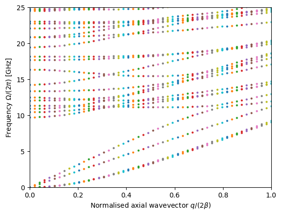
Acoustic dispersion diagram. The elastic wave number \(q\) is scaled by the phase-matched SBS wavenumber \(2\beta\) where \(\beta\) is the propagation constant of the optical pump mode.

5.2.4. Tutorial 4 – Parameter Scan of Widths

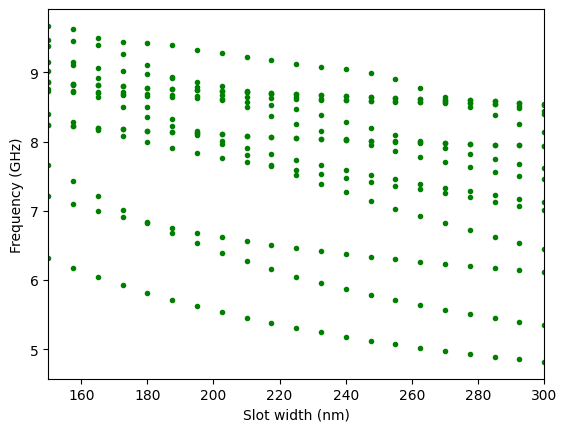
This tutorial, contained in sim-tut_04_scan_widths.py demonstrates the use of a parameter scan of a waveguide property, in this case the width of the silicon rectangular waveguide, to characterise the behaviour of the Brillouin gain. Later examples in the manual show similar calculations expressed as contour plots rather than in this “waterfall” style.

This calculation generates a great many data files. For this reason, we have provided a second argument to the NumBATApp call to specify the name of a new sub-directory, in this case tut_04-out, to store all the generated files.

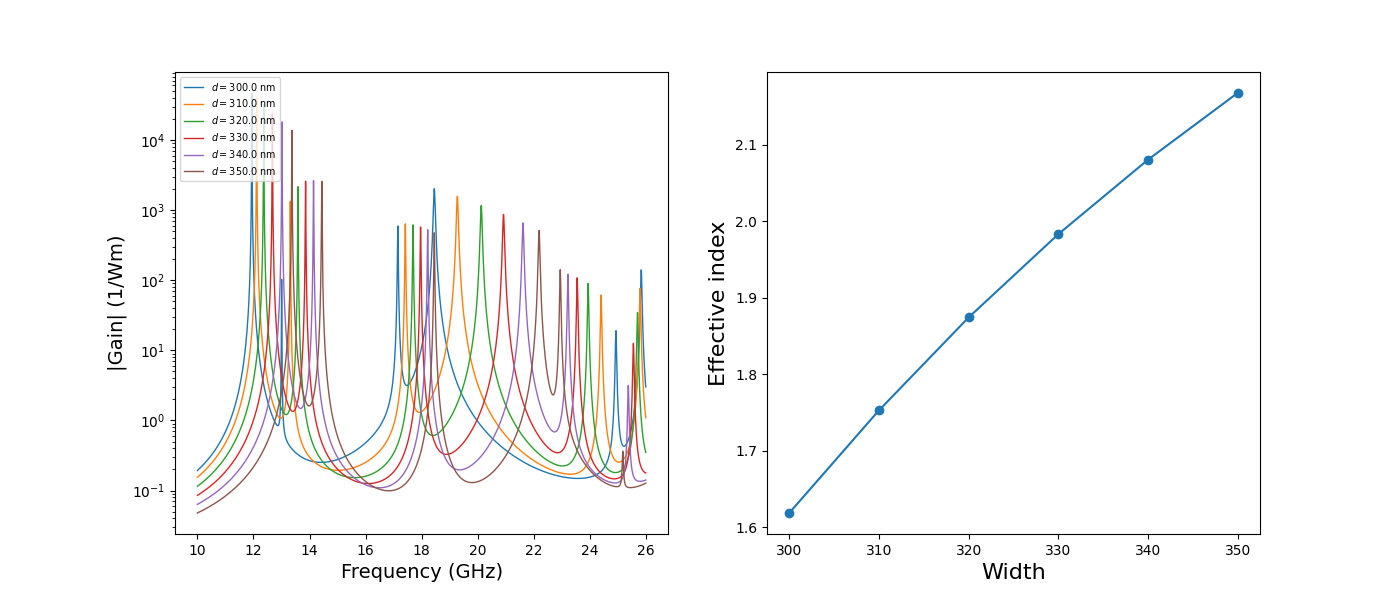
Gain spectra as function of waveguide width.

5.2.5. Tutorial 5 – Convergence Study

This tutorial, contained in sim-tut_05_convergence_study.py demonstrates a scan of numerical parameters for our by now familiar silicon-in-air problem to test the convergence of the calculation results. This is done by scanning the value of the lc_refine parameters. Since these are two-dimensional FEM calculations, the number of mesh elements (and simulation time) increases with roughly the square of the mesh refinement factor.

For the purpose of convergence estimates, the values calculated at the finest mesh (the rightmost values) are taken as the exact values, notated with the subscript 0, eg. \(\beta_0\). The graphs below show both relative errors and absolute values for each quantity.

Once the convergence properties for a particular problem have been established, it can be useful to do exploratory work more quickly by adopting a somewhat coarser mesh, and then increase the resolution once again towards the end of the project to validate results before reporting them.

Convergence of relative (blue) and absolute (red) optical wavenumbers \(k_{z,i}\). The left axis displays the relative error \(|k_{z,i}-k_{z,0}|/k_{z,0}\). The right axis shows the absolute values of \(k_{z,i}\).

Convergence of relative (solid, left) and absolute (chain, right) elastic mode frequencies \(\nu_{i}\).

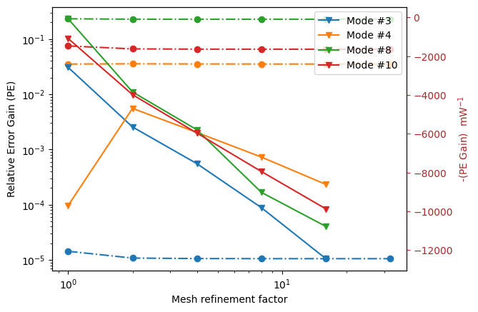
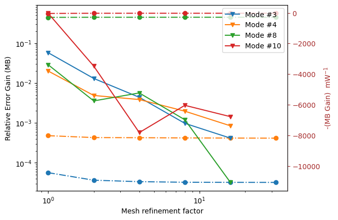
Convergence of photoelastic gain \(G^\text{PE}\). The absolute gain on the right hand side increases down the page because of the convention that NumBAT associates backward SBS with negative gain.

Absolute and relative convergence of moving boundary gain \(G^\text{MB}\).

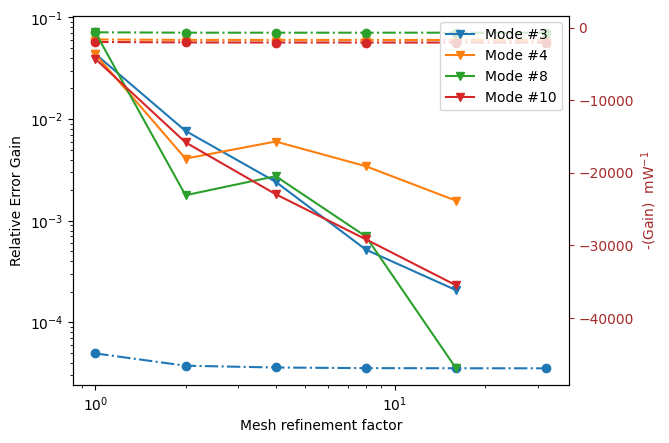
Absolute and relative convergence of total gain \(G\).

5.2.6. Tutorial 6 – Silica Nanowire

In this tutorial, contained in sim-tut_06_silica_nanowire.py we start to explore the Brillouin gain properties in a range of different structures, in this case a silica circular nanowire surrounded by vacuum.

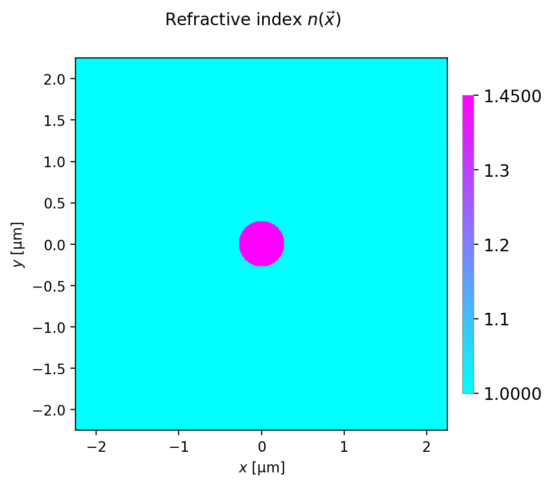
Refractive index profile of the silica nanowire.

The gain-spectra plot below shows the Brillouin gain as a function of Stokes shift. Each resonance peak is marked with the number of the acoustic mode associated with the resonance. This is very helpful in identifying which acoustic mode profiles to examine more closely. In this case, modes 4, , 8 and 23 give the most significant Brillouin gain. The number of modes labelled in the gain spectrum can be controlled using the parameter mark_mode_threshold in the function plot_spectra() to avoid many labels from modes giving negligible gain. Other parameters allow selecting only one type of gain (PE or MB), changing the frequency range (freq_min, freq_max), and plotting with log (logy=True) or dB (dB=True) scales. Note that plots with log scales do not include any noise floor so the peaks look much cleaner than could be observed in the laboratory.

It is important to remember that the total gain is not the simple sum of the photoelastic (PE) and moving boundary (MB) gains. Rather it is the complex coupling amplitudes \(Q_\text{PE}\) and \(Q_\text{MB}\) which are added before squaring to give the total gain. Indeed the two effects may have opposite sign so that the net gain can be smaller than either contribution.

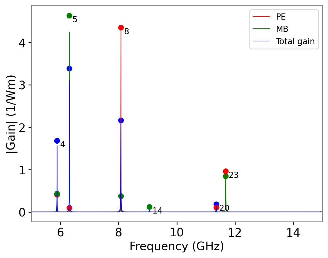
Gain spectrum showing the gain due to the photoelastic effect (PE), the moving boundary effect (PB), and the net gain (Total).

The same data displayed on a log plot using logy=True.

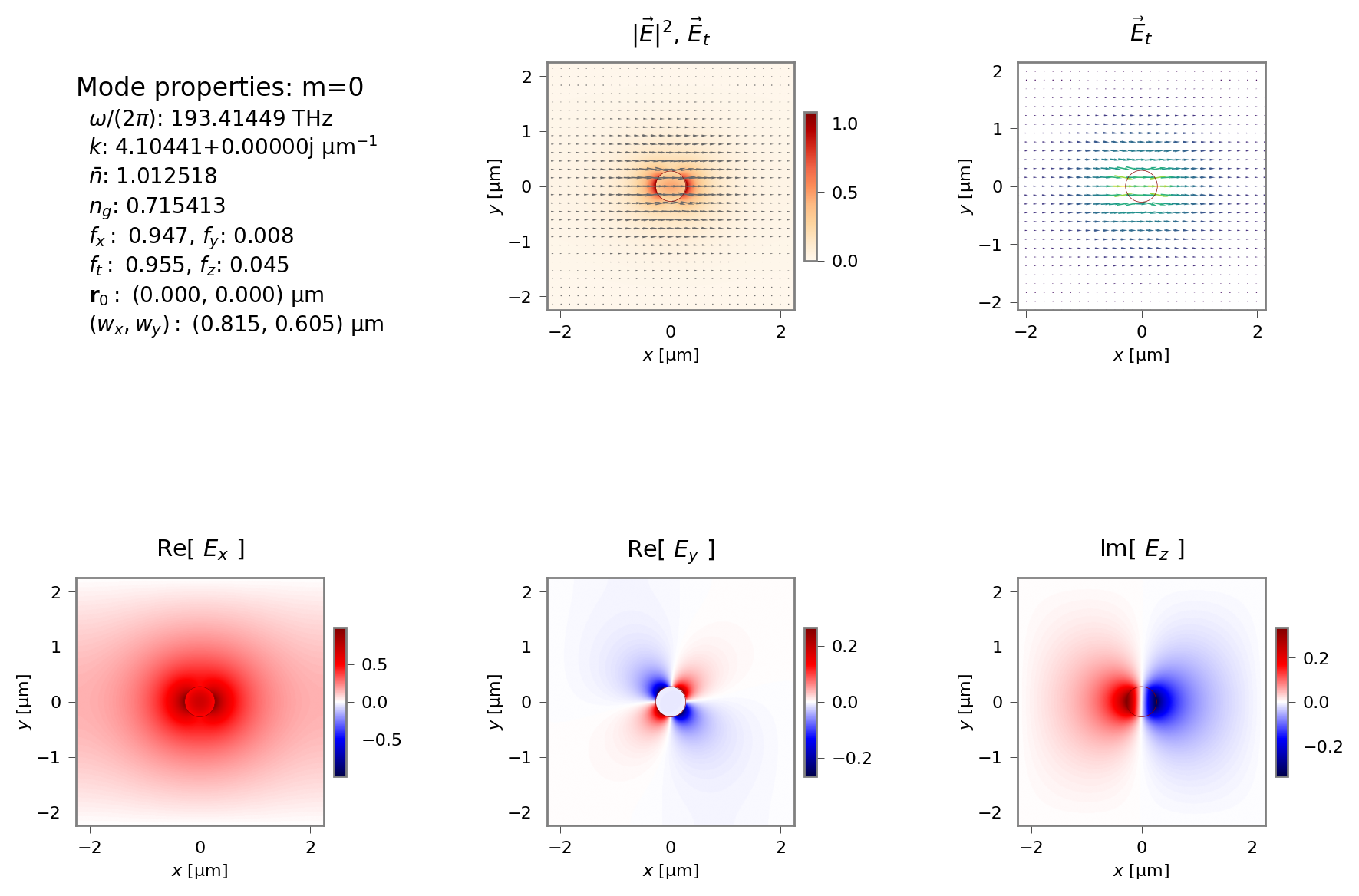
Electromagnetic mode profile of the pump and Stokes field in the \(x\)-polarised fundamental mode of the waveguide.

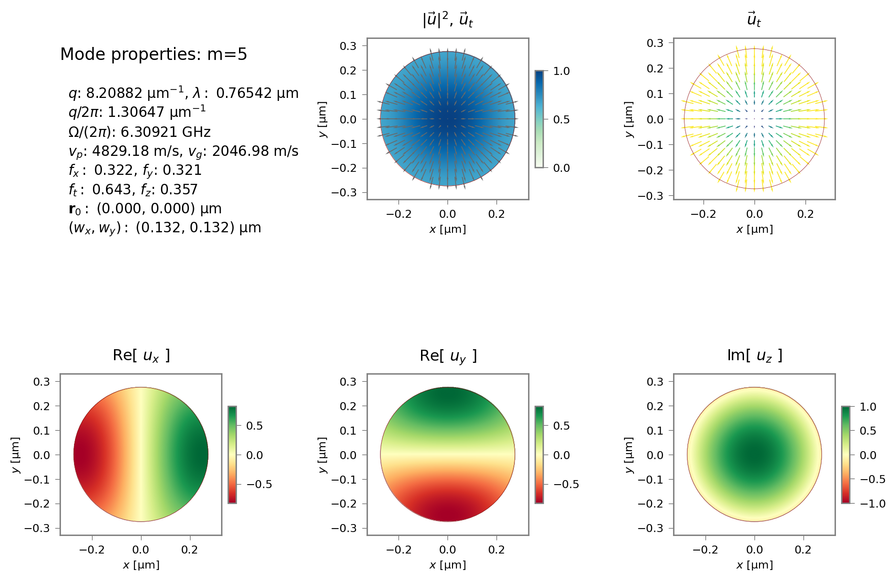
Mode profiles for acoustic mode 5 which is visible as a MB-dominated peak in the gain spectrum.

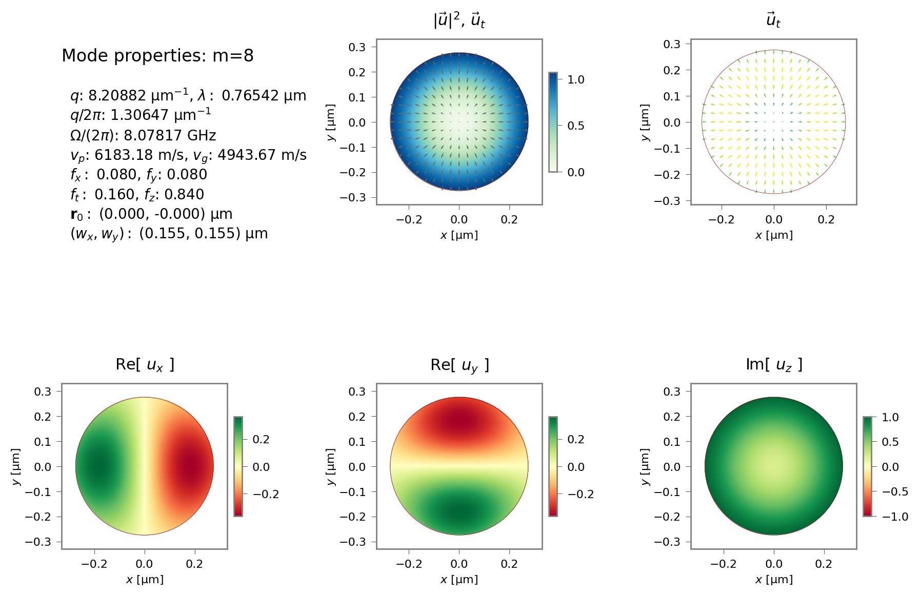
Mode profiles for acoustic mode 8 which is visible as a PE-dominated peak in the gain spectrum.

5.2.7. Tutorial 7 – Slot Waveguide

This tutorial, contained in sim-tut_07-slot.py examines backward SBS in a more complex structure: chalcogenide soft glass (\(\text{As}_2\text{S}_3\)) embedded in a silicon slot waveguide on a silica slab. This structure takes advantage of the slot effect which expels the optical field into the lower index medium, enhancing the fraction of the EM field inside the soft chalcogenide glass which guides the acoustic mode and increasing the gain.

To understand this, it is helpful to see the refractive index and acoustic velocity profiles. Previously, we have seen how to generate images of the Gmsh template and mesh, but that only gives an indirect sense of the final structure.

In this example, we create structure that can plot the refractive index profile and acoustic velocity profile directly. These are created with the calls wguide.get_structure_plotter_refractive_index() and wguide.get_structure_plotter_acoustic_velocity(). Then, on each of these structure we can call one or more methods to generate files containing 1D and 2D profiles. The 1D profiles can be made along any x-cut, any y-cut, or along a straight line between any two points.

In the case of the elastic velocity, since there are in general three phase velocities in each material (in this isotropic case, there are two, corresponding to the longitudinal and shear modes), the 1D profiles include all the velocities, and multiple 2D plots are generated.

Here are a few of these.

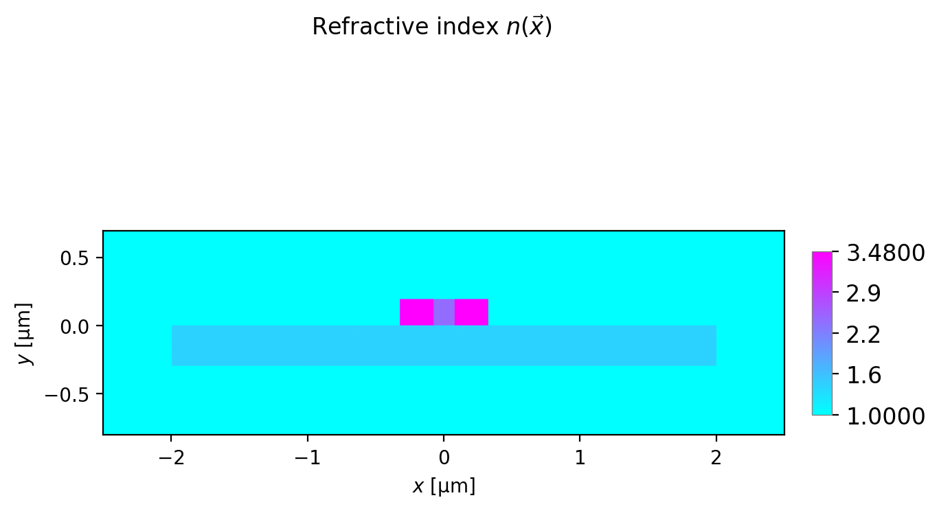
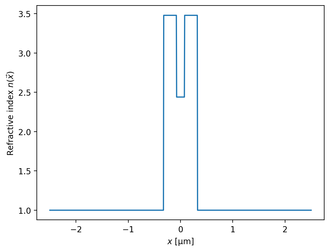
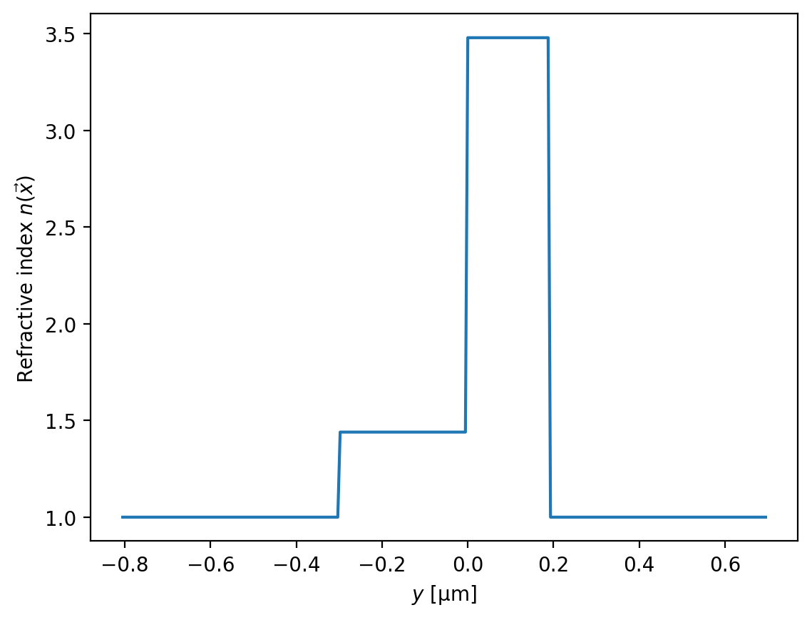
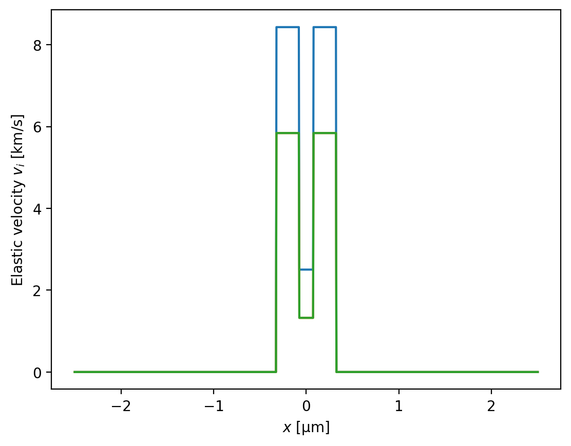
Refractive index profiles (2D, \(x\)-cut at \(y=0.1\), \(y\)-cut at \(x=0.2\) ) of the slot index waveguide.

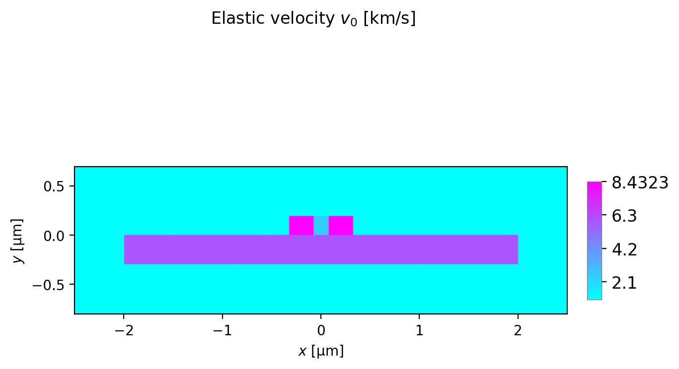
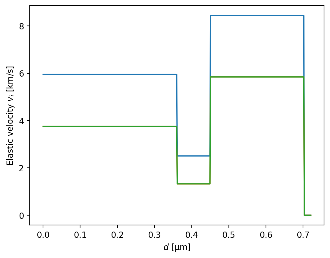
Elastic velocity profiles (2D, \(x\)-cut at \(y=0.1\), 1D slice between the points \((-0.3, -0.2)\) and \((0.3, 0.2)\)) of the slot index waveguide.

Observe that the refractive index is largest in the pillars surrounding the slot and so the optical localisation to the gap region will be via the slot effect. On the other hand, for the elastic problem, both the elastic velocities in the gap are lower than in any other part of the structure, and so we can expect one or more elastic modes truly localised to the slot region by total internal reflection.

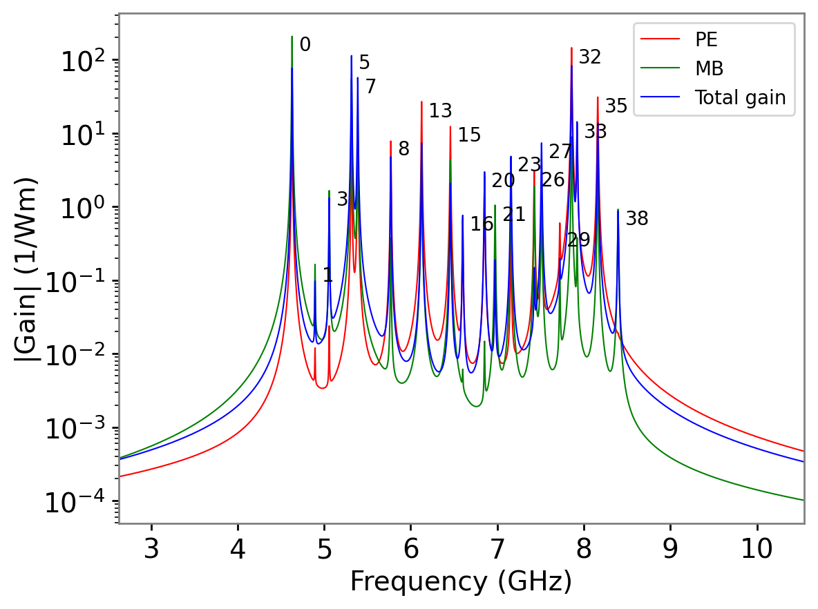
Now we can look at the gain spectra and mode profiles. The highest gain occurs for elastic modes \(m=0\) and \(m=5\).

Gain spectrum showing the gain due to the photoelastic effect (PE), the moving boundary effect (PB), and the net gain (Total).

Gain data shown on a log scale.

Comparing the \(m=0\) and \(m=5\) acoustic mode profiles with the pump EM profile, it is apparent that the field overlap is favourable, whereas the \(m=12\) mode, although being well confined to the slot region, yields zero gain due to its anti-symmetry relative to the pump field.

We also find that the lowest elastic modes are not as localised to the slot region as might be expected. Here, we are seeing a hybridisation of the guided slot mode and Rayleigh-like surface states that are supported on the free boundaries of the slab which is adjacent to the vacuum. This effect could be mitigated by choosing an alternative outer material.

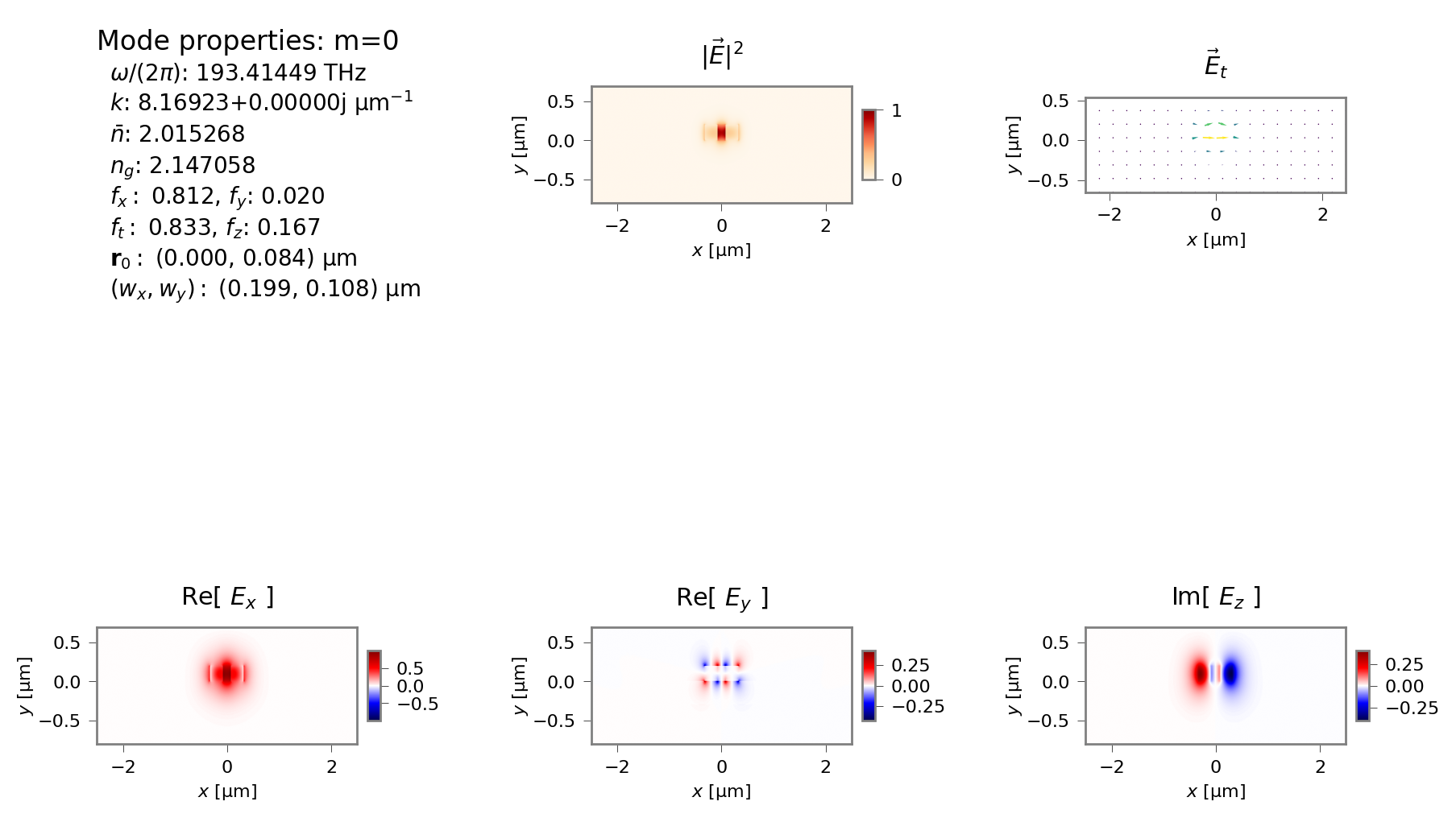
Electromagnetic mode profile of the pump and Stokes field.

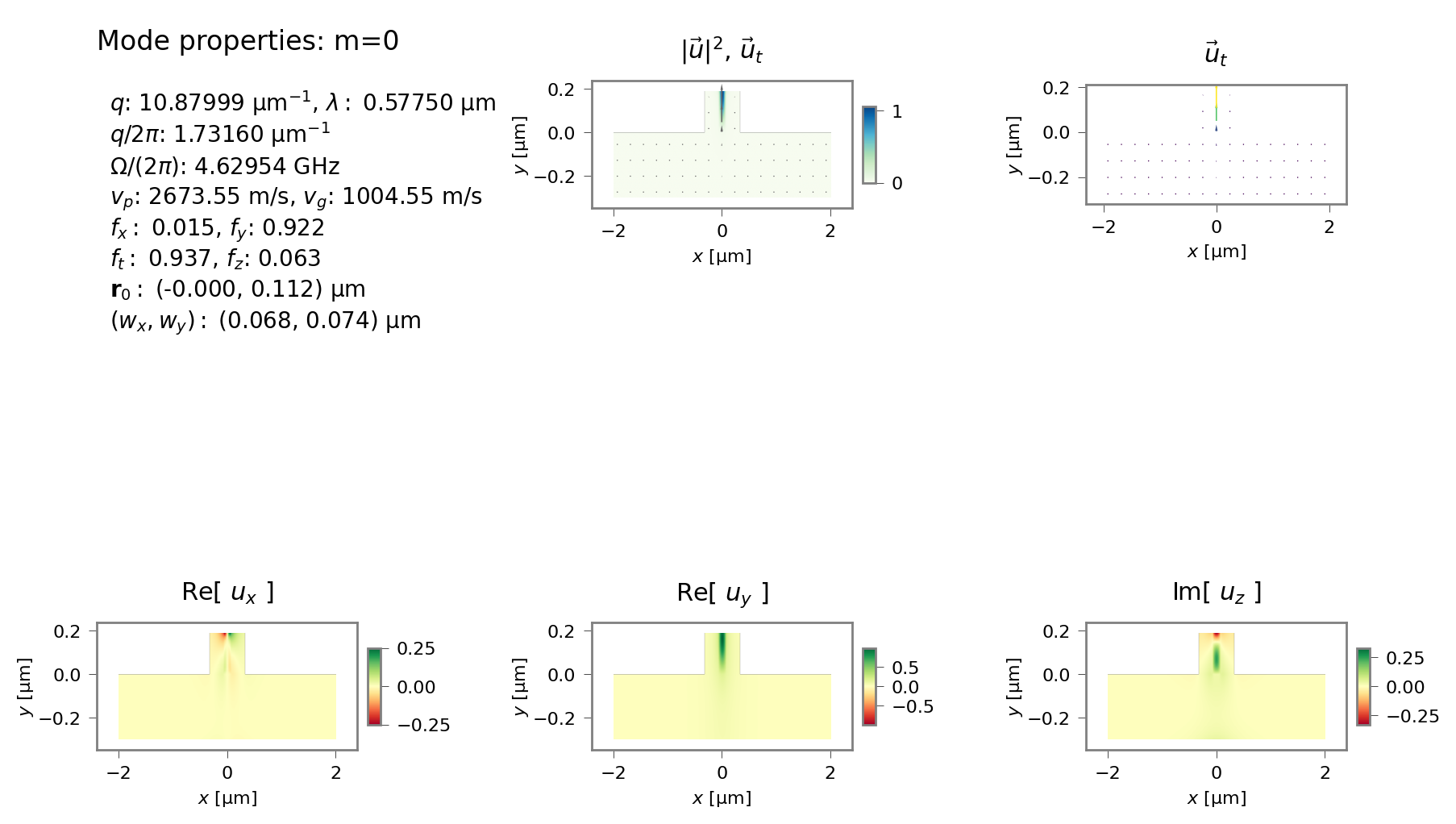
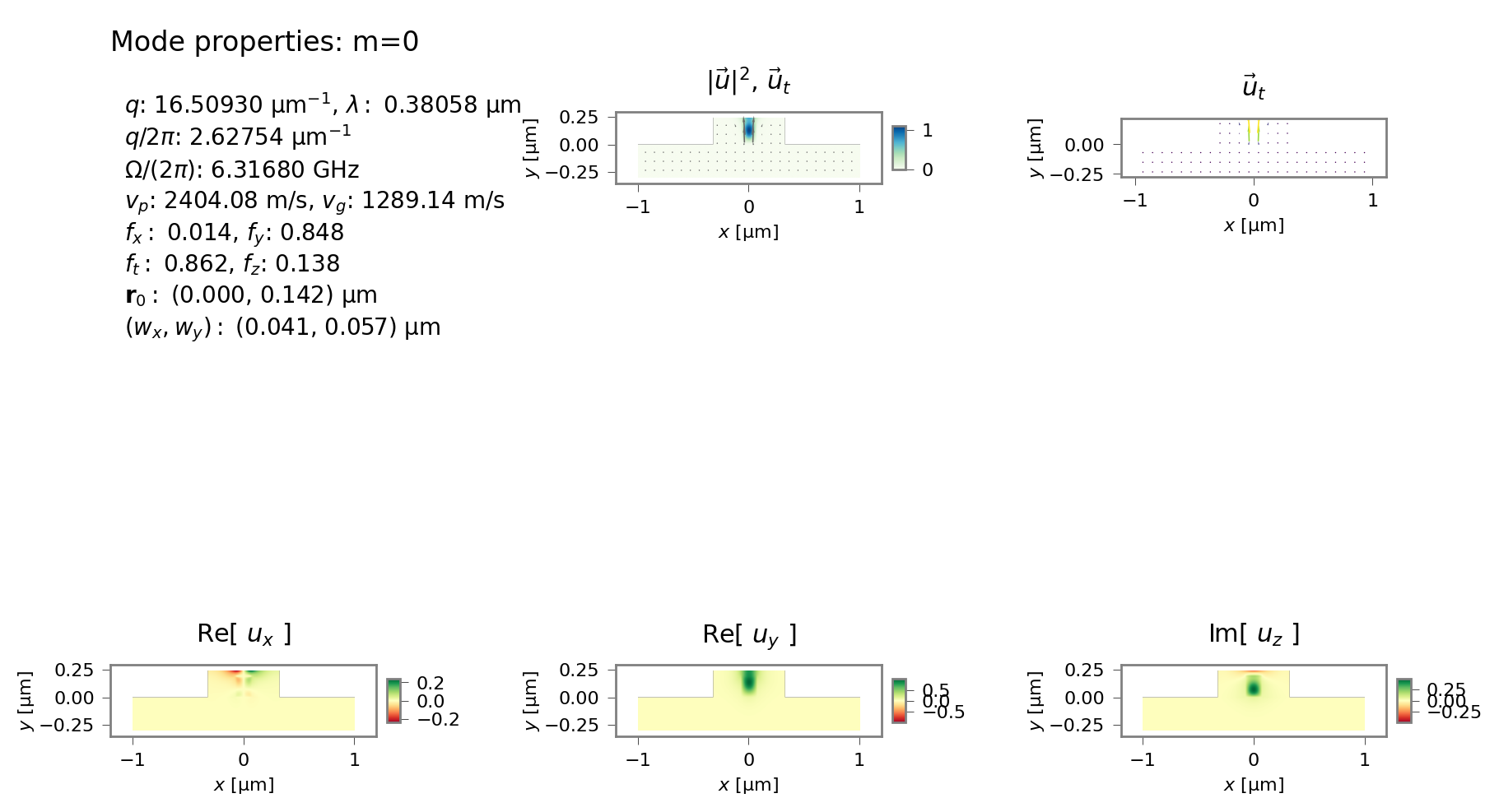
Acoustic mode profiles for mode 0.

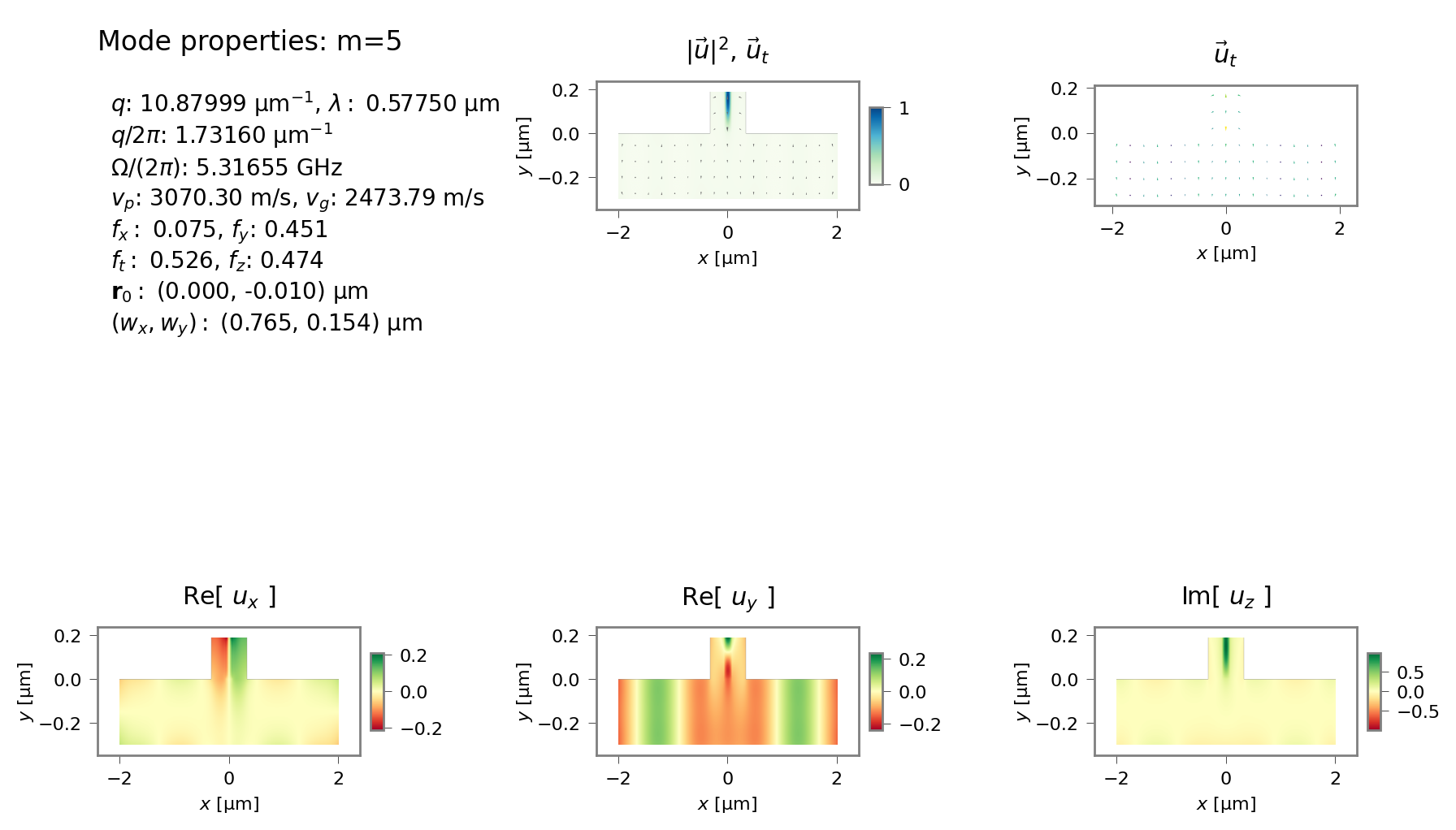
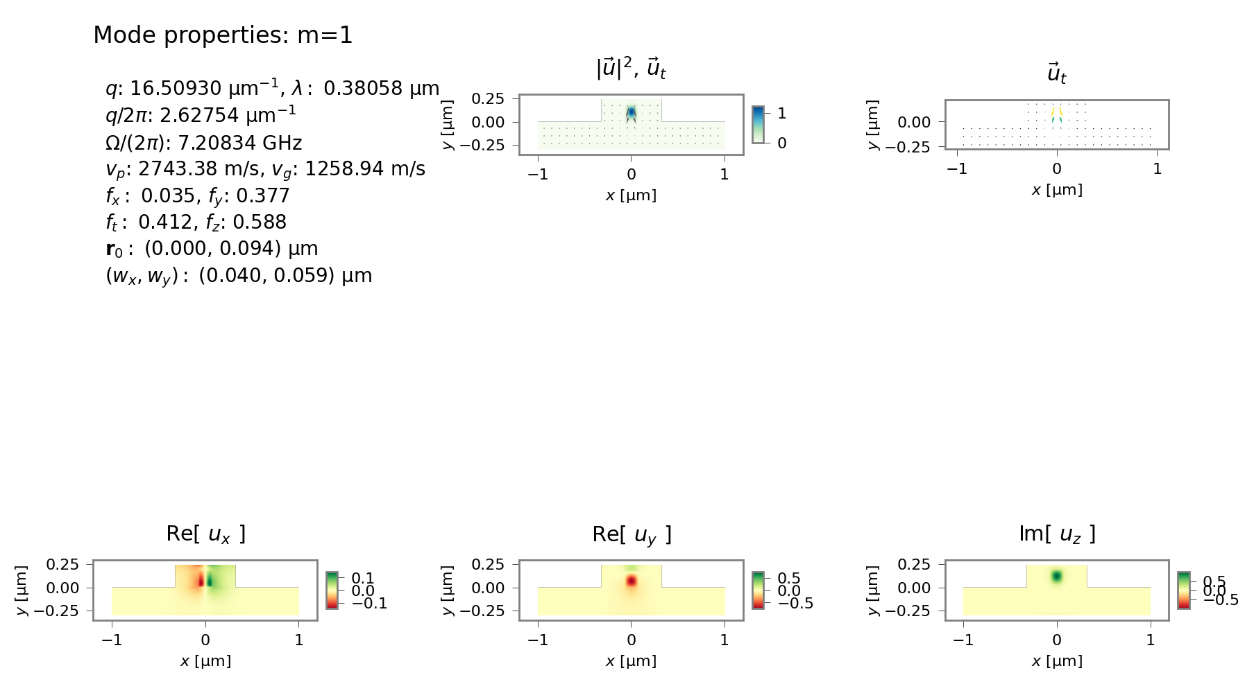
Acoustic mode profiles for mode 5.

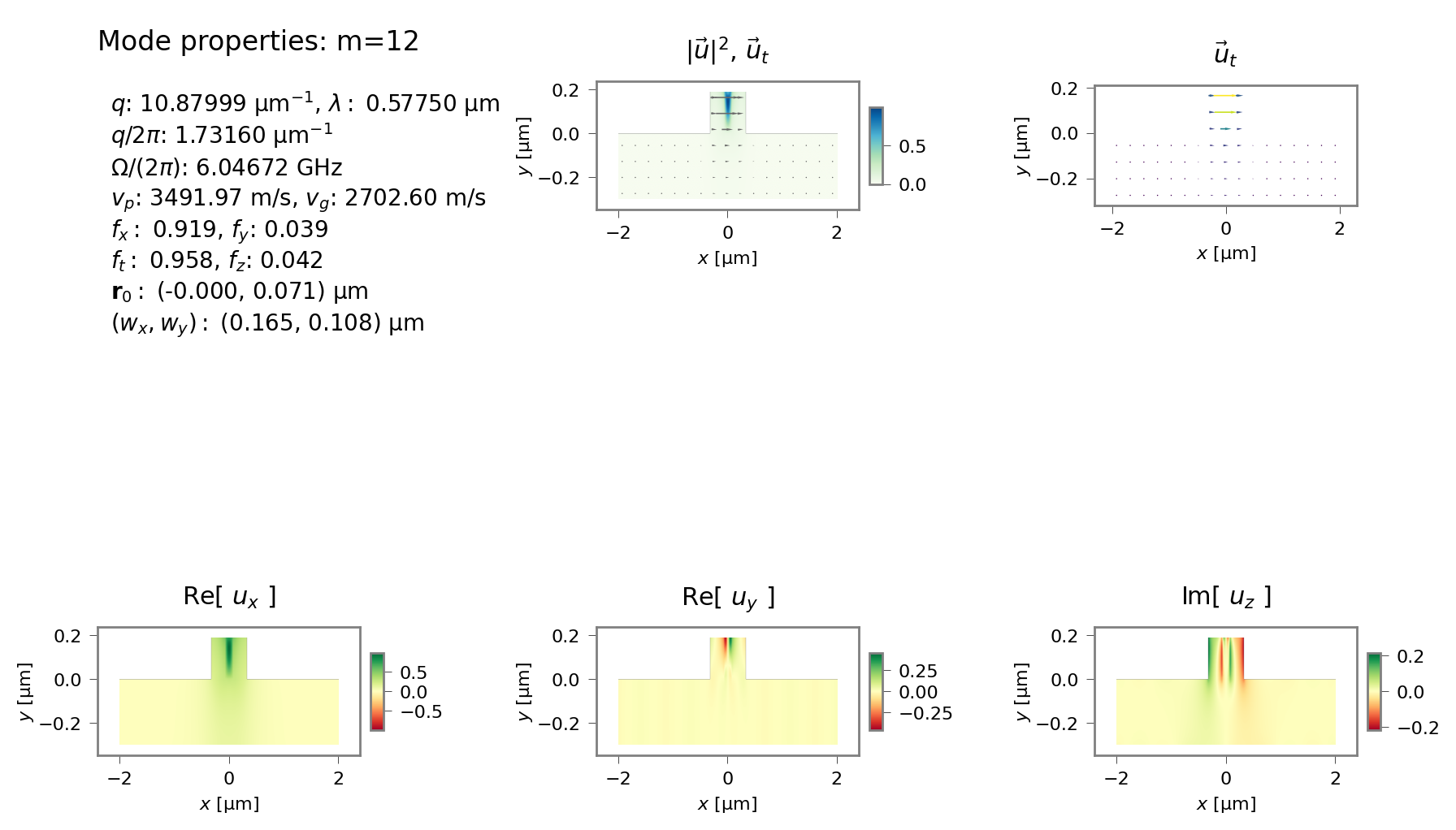
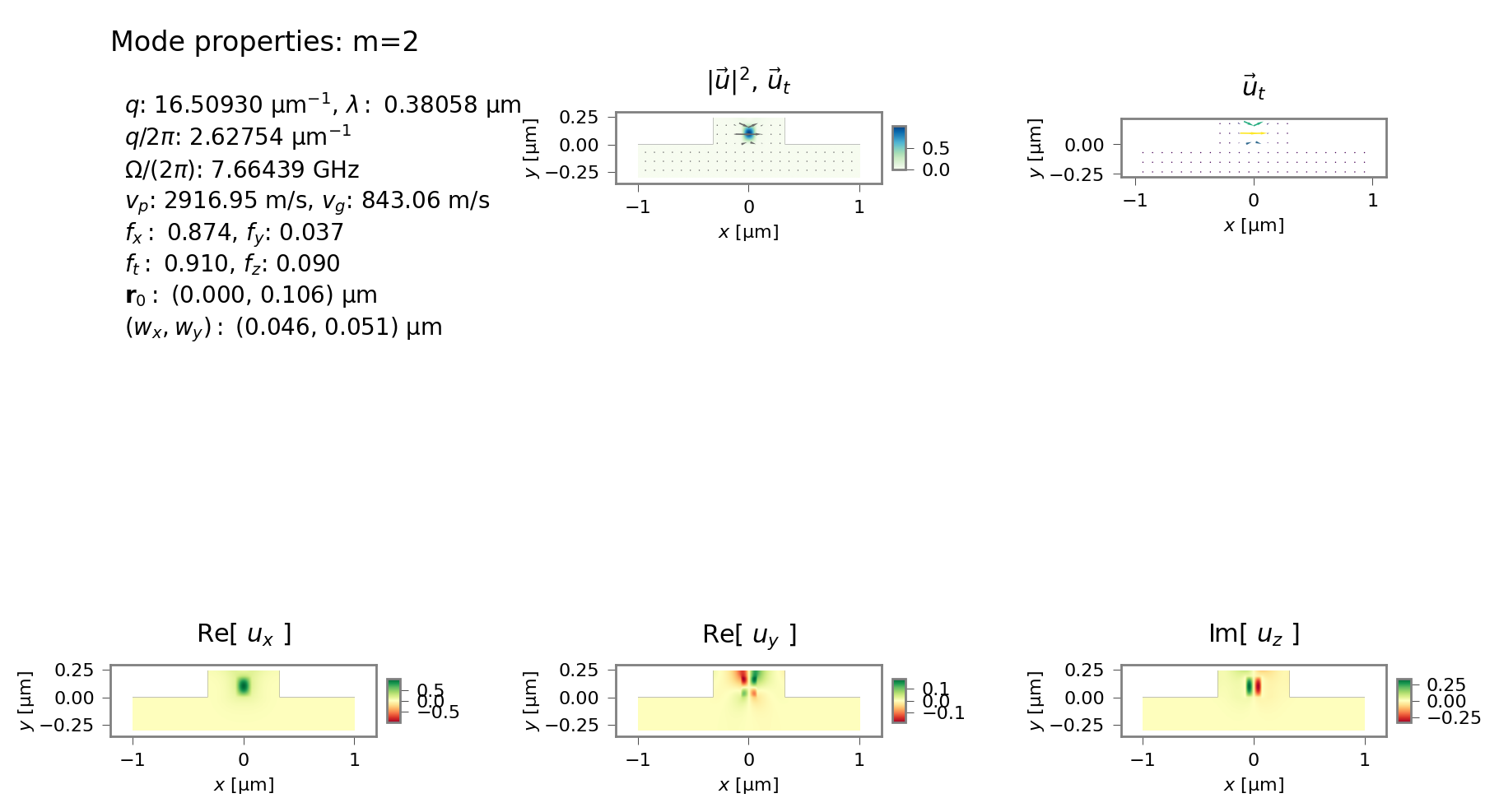
Acoustic mode profiles for mode 12.

Finally, this simulation file includes examples of plots of 1D cut-profiles along different directions. (Look for the plot_modes_1D calls and additional mode outputs in the output fields directory.) Such plots can be useful in resolving features of tightly confined modes.

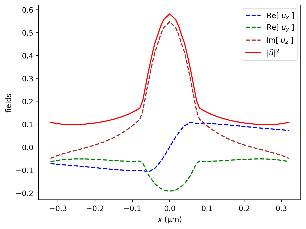
1D y-cut mode profiles for mode 5.

5.2.8. Tutorial 8 – Slot Waveguide Cover Width Scan

This tutorial, contained in sim-tut_08-slot_coated-scan.py continues the study of the previous slot waveguide, by examining the dependence of the acoustic spectrum on the width of the pillars. As before, this parameter scan is accelerated by the use of multi-processing.

The shape of the simulation domain and the compactness of the mode makes the default mode displays hard to see clearly. While this can be addressed with plot settings such as the aspect ratio, and number of vector arrows, it is also helpful to plot each component separately on its own plot. this is achieved with the comps option to plot_modes().

Acoustic frequencies as function of covering layer thickness.

Modal profiles of lowest acoustic mode.

Modal profiles of second acoustic mode.

Modal profiles of third acoustic mode.

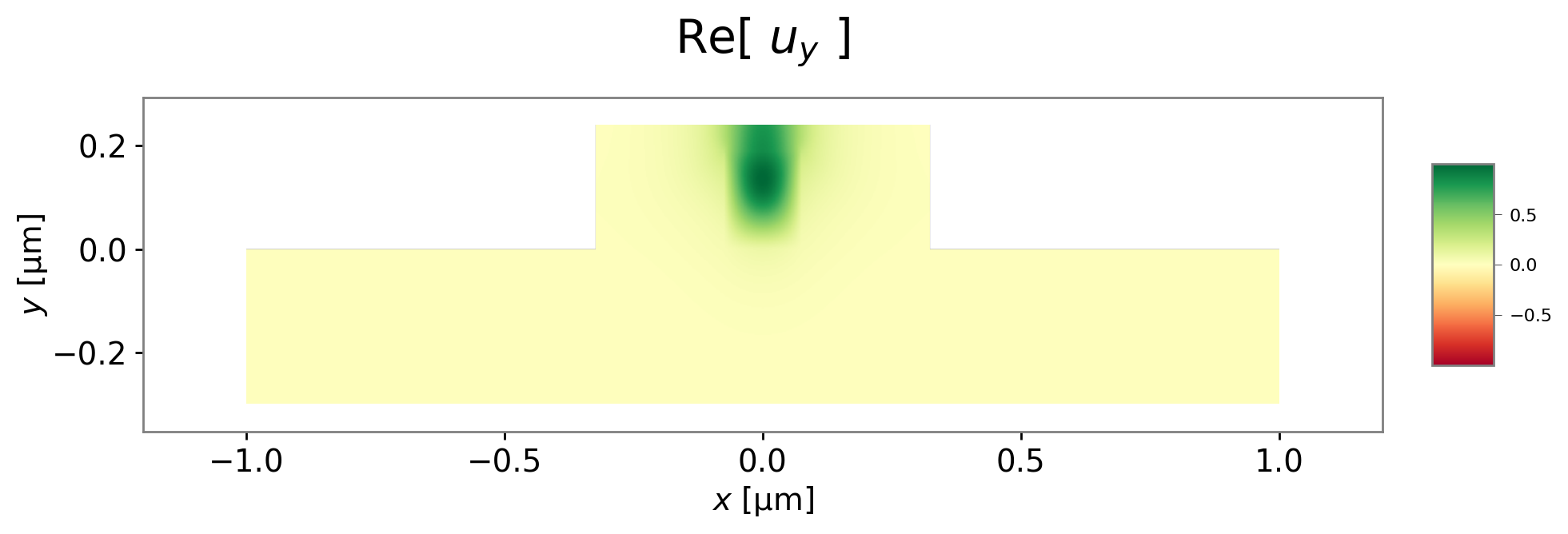
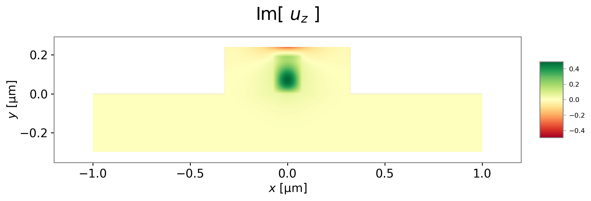
Individual components of the lowest acoustic mode.